বইগুলো এখনো বাংলা ভাষায় পাওয়া যায় না — ইংরেজি সংস্করণ দেখানো হচ্ছে।
University Earth and Space Sciences — Year 1 · স্নাতক প্রথম বর্ষ
26Structure of the Atmosphere and the Ocean
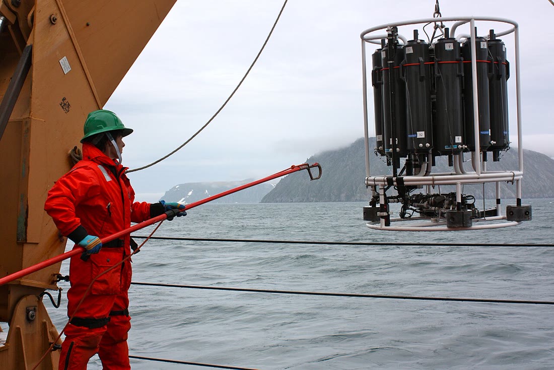
Twice a day, at weather stations around the world, a balloon is released carrying a radiosonde, a small instrument that radios back the pressure, the temperature and the humidity of the air as it rises; it climbs at about a minute and can pass before the balloon bursts. Far out at sea, a research ship lowers a frame of instruments and water bottles on a cable to the abyss, measuring the conductivity, the temperature and the depth all the way. The two profiles, one of the air and one of the water, are the raw material of this chapter. Both envelopes are layered, and in both the layering is set by density: light fluid above heavy fluid. What makes a layer light or heavy is less obvious than it looks. Air that is colder than the air below it can still be the lighter; water that is warmer than the water above it can still be the heavier. The chapter builds the two tools that sort this out, the potential temperature and the equation of state of seawater.
You already know
The physics volumes give the hydrostatic relation, , for a fluid at rest; for an ideal gas of molar mass , , and in an isothermal atmosphere the pressure falls as with the scale height . They state the first law for a closed system and, for an ideal gas, Laplace’s relation along a reversible adiabatic transformation, constant, with and per unit mass. A body immersed in a fluid receives an upward thrust equal to the weight of fluid it displaces (Archimedes). Book 1 named the layers of the atmosphere and the environmental lapse rate of the standard atmosphere, per kilometre in the troposphere; Book 2 admitted the dry adiabatic rate, per kilometre, called air stable or unstable according to the fate of a parcel pushed upwards, and described the mixed layer, the thermocline, the halocline and the pycnocline of the ocean. The salinity of seawater is close to 35 grams of dissolved salts per kilogram.
26.1 The vertical structure of the atmosphere
No real sounding is the same as the next one. To compare them, a reference profile is fixed by convention.
Definition 26.1 (Standard atmosphere)
A standard atmosphere is a profile of temperature, pressure and density against height fixed by convention: dry air of constant molar mass, an ideal gas in hydrostatic balance, with given values at sea level and a temperature that varies linearly with height in successive layers. The 1976 standard atmosphere takes and at sea level, , and .
Below the 1976 standard has four layers (Table 26.1). The lowest, the troposphere, cools at per kilometre; from its top, the tropopause, the temperature stays at for nine kilometres, then rises. The heights of the standard are geopotential heights, the heights that a constant gravity would give the same potential energy; below they differ from geometric heights by less than ( of the standard lie at ).
| Layer | Base (km) | (K/km) | at base (K) | at base (hPa) |
|---|---|---|---|---|
| 1 (troposphere) | 0 | 288.15 | 1013.25 | |
| 2 (stratosphere) | 11 | 0.0 | 216.65 | 226.32 |
| 3 (stratosphere) | 20 | 216.65 | 54.75 | |
| 4 (stratosphere) | 32 | 228.65 | 8.68 |
In each layer the temperature is a linear function of height, so the hydrostatic relation can be integrated in closed form.
Proposition 26.2 (Pressure in a layer of constant gradient)
In a layer of dry air where with a constant , the pressure is
where and are the values at the base . When the pressure falls exponentially with the scale height .
Proof. The hydrostatic relation and the ideal gas give . Since , this is , which integrates to . For , and : the isothermal atmosphere of the physics volumes. ∎
In the troposphere of the standard, , and at , K: , a little under a quarter of the sea-level value. In the isothermal layer above, , and nine kilometres higher the pressure has fallen by a further factor , to . Since the pressure at a level is the weight, per unit area, of the air above it, half of the mass of the standard atmosphere lies below and nine tenths below .
26.2 Lapse rates and potential temperature
Definition 26.3 (Environmental and dry adiabatic lapse rates)
The environmental lapse rate is , the rate at which the temperature of the air at rest decreases with height, as a sounding measures it. The dry adiabatic lapse rate is the rate at which the temperature of a parcel of unsaturated air decreases as the parcel is lifted.
A lapse rate is positive when the temperature falls with height. The two rates are of different natures: the first describes the state of the atmosphere at one moment; the second, the transformation of a piece of air that moves.
Definition 26.4 (Air parcel)
An air parcel is a volume of air followed in its motion, small enough to have a single temperature and pressure and not to disturb the air around it, large enough to keep its identity: it exchanges no mass and, during a quick displacement, no heat with its surroundings, and its pressure is at every moment that of the surrounding air.
The parcel is an idealisation, like the closed system of thermodynamics: the results below hold for real air to the extent that a moving piece of it exchanges little heat and little mass with its surroundings.
Theorem 26.5 (The dry adiabatic lapse rate)
A parcel of dry air, lifted adiabatically and reversibly through air at rest of nearly the same temperature, cools at the rate
where is the specific heat of air at constant pressure. With , .
Proof. For a kilogram of the parcel, of temperature and density , the first law of a reversible transformation without heat exchange, written with the enthalpy, is . The pressure of the parcel is that of the air around it, which is hydrostatic: , with the density of the surrounding air. Hence
since at equal pressure the densities of two ideal gases of the same molar mass are in the inverse ratio of their temperatures. When the parcel is at nearly the temperature of its surroundings, and . For dry air, an ideal diatomic gas, , so , and . ∎
A parcel warmer than its surroundings, near , cools at , faster; the correction is neglected in what follows. The rate does not depend on the pressure or the temperature of the parcel, and a parcel that sinks warms at the same rate, as Book 2 followed air over a mountain.
Integrating the same equation without the hydrostatic step gives a quantity that the parcel carries with it.
Proposition 26.6 (Potential temperature)
Along a reversible adiabatic transformation of dry air,
stays constant, whatever the reference pressure .
Proof. From and , , so is constant, and so is ; multiplying by the constant gives . This is Laplace’s relation written with and . ∎
Definition 26.7 (Potential temperature)
The potential temperature of a parcel of dry air is the temperature it would have if brought adiabatically to the reference pressure : with in hectopascals and in kelvins.
The potential temperature is a label that a dry parcel keeps when it rises or sinks without exchanging heat, as the salinity of a water parcel is. Heating by radiation, by condensation of water or by mixing changes it; the rest does not.
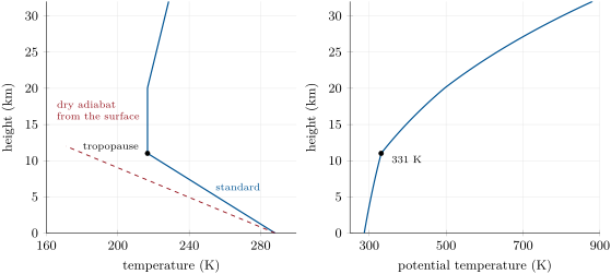
Example 26.8 (The tropopause of the standard atmosphere)
At the surface of the standard, . At the tropopause, and : . Air from the tropopause brought down adiabatically to would arrive at , warmer than surface air brought to the same pressure. The temperature falls by from the ground to the tropopause, yet the potential temperature rises by .
26.3 Static stability
Definition 26.9 (Static stability; temperature inversion)
The static stability of a layer at rest is its response to a small vertical displacement of a parcel. The layer has a stable stratification if the displaced parcel is pushed back towards its level, an unstable stratification if it is pushed further away, and a neutral stratification if no force acts on it. A temperature inversion is a layer in which the temperature increases with height.
Theorem 26.10 (The criterion of static stability)
A layer of dry air at rest, of temperature and environmental lapse rate , is stable if , neutral if and unstable if ; equivalently, it is stable if and only if its potential temperature increases with height. A parcel displaced by a small in a stable layer oscillates about its level at the angular frequency , where
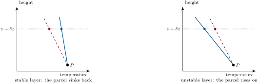
Proof. A parcel at the temperature of its level is lifted by . It arrives at , while the air around it is at . Per unit mass, the parcel feels its weight and the thrust of Archimedes, a net upward acceleration , the pressures being equal. To first order in this is
If , and the parcel oscillates at the angular frequency ; if the displacement grows exponentially; if no force acts. For the second form, take the logarithmic derivative of and use the hydrostatic relation:
since . ∎
The angular frequency is called the buoyancy frequency. In the troposphere of the standard, near the ground, , , and the period of the oscillation is about . In the isothermal lower stratosphere : , twice as large, a period of five minutes. The stratosphere is a lid: it resists vertical motion much more strongly than the troposphere below it.
On a diagram of temperature against height, the criterion compares two slopes (figure below): the parcel follows the dry adiabat through its starting point, and the question is on which side of the sounding it finds itself after a small displacement.
Method 26.11 (Reading the stability of a sounding)
- Divide the sounding into layers between levels where the slope changes.
- In each layer compute , in kelvins per kilometre.
- Compare with : unstable, close to neutral, stable; a negative is an inversion, the most stable case.
- Where pressures are given rather than heights, compute at each level: decreasing upwards marks an unstable layer, constant a neutral one, increasing a stable one.
An unstable layer does not last: a displacement in it grows exponentially, at the rate , and the parcels it releases overturn it, mixing it until its potential temperature is uniform and its lapse rate is . A layer heated from below, by warm ground or a warm sea, is pushed towards instability; one cooled from below, towards stability. An inversion caps whatever lies below it: a parcel rising from below finds itself colder than its surroundings as soon as it enters it. Above the whole stratosphere of the standard is an inversion.
All of this assumes dry air. A rising parcel that becomes saturated releases latent heat as its water condenses and cools more slowly than ; the saturated adiabat and the conditional instability it brings are the subject of next year’s volume.
26.4 The layered ocean
The ocean exchanges heat and water with the atmosphere only at its surface, through heating and cooling, evaporation and rain. Its vertical structure has three ingredients, temperature, salinity and density.
Definition 26.12 (Mixed layer, thermocline, halocline, pycnocline)
The mixed layer is the surface layer of the ocean whose temperature, salinity and density are nearly uniform with depth; its depth is read on a profile as the depth where the temperature first differs from its surface value by a chosen threshold, often . The thermocline, the halocline and the pycnocline are the layers below it in which the temperature, the salinity and the density respectively change fastest with depth.
The pressure in the ocean is quoted in decibars, because one decibar, , is nearly the pressure of one metre of seawater: at of latitude, lie at and at .
Water is nearly incompressible, but not quite, and a parcel of water brought up from the deep expands and cools a little, as a parcel of air does. The adiabatic lapse rate of seawater is small, about per at the surface at and per at , against per kilometre in air; but over five kilometres it adds up to a few tenths of a degree, more than the differences between deep waters. Oceanographers therefore compare waters by their potential temperature too: the temperature a parcel would have if raised adiabatically, without change of salinity, to the surface. A water of at and salinity 35 has a potential temperature of . In the deepest levels of the South Atlantic at , the measured temperature rises from at to at while the potential temperature falls from to : the warming is compression, not heat.
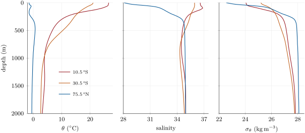
The three columns of the figure above show the three kinds of upper ocean. In the tropics, a warm mixed layer near sits on a sharp thermocline: between and the potential temperature drops from to , and the density follows it, so the thermocline is also the pycnocline. At the surface is cooler, , and the fall more gradual, spread over the upper . In both, salinity is highest near the surface and decreases downwards; it works against the stratification, which the temperature more than makes up for. The Arctic column is the opposite case. Its surface water, at , is the coldest of the three, yet the lightest, , because its salinity is only ; salinity rises to at . The halocline is the pycnocline here. Below it lies a layer warmer than the water above, near at : a temperature inversion that is perfectly stable, held down by its salt.
26.5 Seawater density and T–S diagrams
Definition 26.13 (Equation of state of seawater; haline contraction coefficient; density anomaly)
The equation of state of seawater gives its density as a function of salinity, temperature and pressure. The haline contraction coefficient is at constant temperature and pressure. The density anomaly is a density minus : uses the measured temperature at zero sea pressure, and the potential density anomaly the potential temperature.
The equation of state is not derived from first principles but fitted to laboratory measurements. The international equation of 1980 at the pressure of the surface is a polynomial with fifteen coefficients, , where is the density of pure water; it gives . A thermodynamic description of seawater, TEOS-10, was adopted in 2009 to replace it as the official one; the 1980 equation is used here because its polynomial fits on a page. Its thermal expansion coefficient is the coefficient of the physics volumes.
| () | () | () | |
|---|---|---|---|
| 0 | 1028.106 | ||
| 10 | 1026.952 | ||
| 25 | 1023.343 |
The expansion coefficient is six times larger in warm water than in water near freezing, while hardly changes (Table 26.2). One unit of salinity weighs as much as about at , but as much as near : in cold polar water, density is set by salinity, as the Arctic column showed.
Proposition 26.14 (Linear equation of state)
Near a reference state of density , at fixed pressure,
with and evaluated at the reference state; the error is of second order in and .
Proof. This is the first-order Taylor expansion of at , since and there. ∎
About the linear form gives the density of water at within , but that of a surface water at too high: the equation of state is curved, and its curvature has consequences.
Definition 26.15 (T–S diagram; water mass)
A T–S diagram is a plot of the potential temperature of the samples of a profile against their salinity, with the depths written along the curve and the lines of equal drawn underneath. A water mass is a body of water with a common formation history, recognised by its range of potential temperature and salinity.
A water mass acquires its temperature and salinity at the surface, through heating and cooling, evaporation and rain, in the region where it forms; once it sinks below the mixed layer, out of contact with the atmosphere, it can change them only by mixing with its neighbours. Potential temperature and salinity are then tracers.
Proposition 26.16 (Mixing lines are straight)
When masses and of two waters and mix completely, the mixture has
on a T–S diagram it lies on the segment joining the two waters, at distances from them in the inverse ratio of their masses. Mixtures of three waters fill the triangle they form.
Proof. The salinity is a mass fraction of salt, and salt is conserved: the mass of salt in the mixture, , divided by its mass, gives . Mixing at constant pressure conserves the enthalpy; with a specific heat that varies little, this is a weighted mean of the potential temperatures, to within a relative error of about per unit of salinity difference. The point is then the barycentre of the two points with the weights and . ∎
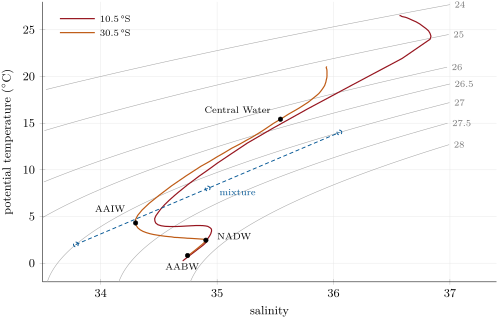
The two South Atlantic columns draw the same figure on the T–S diagram: the similarity of curves from places far apart is what reveals water masses. From the surface down to about , the curves follow a nearly straight line, steep in temperature: this is Central Water, which fills the upper kilometre of the subtropical ocean. Below it, both curves turn to a salinity minimum, at and at : Antarctic Intermediate Water (AAIW), formed under the rainy westerlies of the Southern Ocean, sinking to about and spreading north. Deeper, a salinity maximum, at : North Atlantic Deep Water (NADW), formed in the Greenland and Labrador Seas, sinking to about and moving south through the whole Atlantic. At the bottom the curves converge on the coldest water, at : Antarctic Bottom Water (AABW), formed along the Antarctic continent, which fills the oceans below about . At the salinity minimum lies at and the maximum at , with a higher maximum, : the NADW is closer to its source there.
The extremes are themselves mixing products. AAIW, as it moves north, mixes with the saltier water above and below it; by Proposition 26.16 its core moves towards them on the diagram and the minimum erodes. A salinity minimum or maximum on a profile is always the trace of a water that came from elsewhere, carried sideways at its own density level.
Method 26.17 (Reading water masses on a T–S diagram)
- Convert the measured temperatures to potential temperatures (in the upper kilometre the difference is below and may be neglected).
- Plot against , writing the depths along the curve.
- Read the straight segments as mixtures of the two waters at their ends, the extremes of salinity or temperature as the cores of water masses, and the end of the curve near the bottom as the densest water present.
- Read the density on the isopycnals: along a stable profile, increases with depth.
Because the isopycnals are curved, two waters of the same density do not mix to a water of that density. Water at and water at both have ; mixed in equal parts, they give , of (figure above). The mixture is denser than both parents and sinks below them. This densification on mixing, called cabbeling, is the cost of the curvature of the equation of state: with the linear form of Proposition 26.14, the density of a mixture would be the mean of the densities. Along the isopycnal surfaces of the ocean, where eddies stir waters of different temperature and salinity, cabbeling drives a slow sinking across them.
A last caution. Referred to the surface, the AABW at comes out at , slightly lighter than the NADW above it, ; at the bottom of the column at , even decreases downwards. The ratio of the equation of state changes with pressure, so that the order of two waters of different temperatures can depend on the pressure at which their densities are compared. Waters thousands of metres deep are compared with a density referred to a pressure nearer their own, such as , referred to ; the method is that of next year’s volume.
26.6 Exercises
Exercise 26.1 ★
(a) Compute the scale height of air at with the constants of the standard atmosphere. (b) By what factor does the pressure fall over in an isothermal layer at that temperature? (c) Why is the scale height smaller at the tropopause than at the ground?
Solution
Solution of Exercise 26.1.
(a) . (b) : the pressure falls to about a quarter. (c) is proportional to the temperature: at it is , against at . Cold air is denser at a given pressure, so the pressure falls faster with height.
Exercise 26.2 ★
A sounding gives, in kelvins per kilometre, the lapse rates (), (), (), () and (above ). Classify each layer as unstable, neutral, stable or an inversion, and say which is the most stable.
Solution
Solution of Exercise 26.2.
With : , , unstable; , , neutral to within the precision of the data; , an inversion; , stable; above , isothermal, stable. The inversion is the most stable, since is largest there.
Exercise 26.3 ★
(a) Seawater has a density of . What is its density anomaly? (b) Of two waters, A with and B with , which lies above the other when both are at rest in the same column? (c) Why do oceanographers write rather than ?
Solution
Solution of Exercise 26.3.
(a) . (b) B, the lighter, lies above A. (c) All seawater densities begin with the same digits, 10; keeps only the digits that change from one water to another.
Exercise 26.4 ★
Water P mixes with water Q . (a) Compute the salinity and the potential temperature of a mixture of one part of P with three parts of Q. (b) Where does it lie on the T–S diagram? (c) A third water R is added. Can the mixture of the three have ?
Solution
Solution of Exercise 26.4.
(a) ; . (b) On the segment PQ, a quarter of the way from Q to P (Proposition 26.16). (c) The mixtures of P, Q and R fill the triangle PQR. Writing with gives , , : a negative proportion of R, so the point lies outside the triangle and no mixture of the three can produce it.
Exercise 26.5 ★★
(a) At the air is at . Compute its potential temperature. (b) At the ground, at , the air is at . Is the layer between the two stable for dry air? (c) What would be the temperature of the air brought down adiabatically to the ground?
Solution
Solution of Exercise 26.5.
(a) . (b) At , . The potential temperature increases upwards, from 298.2 to : the layer is stable for dry air. (c) It would arrive at its potential temperature, , that is , ten degrees warmer than the air already there.
Exercise 26.6 ★★
(a) With Proposition 26.2, compute the pressure at in the standard atmosphere. (b) Compute it again assuming an isothermal atmosphere at . Which is lower, and why? (c) Compute the pressure at from the values at of Table 26.1.
Solution
Solution of Exercise 26.6.
(a) and , . (b) and . The real (standard) pressure is lower: the air there is colder than , hence denser, and the pressure falls faster with height. (c) , the value of Table 26.1.
Exercise 26.7 ★★
Use the linear equation of state about with the coefficients of Table 26.2. (a) What change of salinity compensates, for the density, a warming of ? (b) A water at is warmed by and made saltier by . Does it become denser or lighter, and by how much? (c) Answer the same question for a water at , with the coefficients of that temperature.
Solution
Solution of Exercise 26.7.
(a) gives . (b) : the water becomes lighter. (c) : the same changes now make it denser, because warming barely changes the density of water near freezing.
Exercise 26.8 ★★
A layer at has a lapse rate of . (a) Compute its buoyancy frequency and the period of the oscillation of a parcel displaced in it. (b) Compute the same quantities for an inversion at where . (c) What happens to the period as approaches ?
Solution
Solution of Exercise 26.8.
(a) , , period , about seven minutes. (b) , , period . (c) tends to zero and the period grows without bound: the restoring force vanishes in a neutral layer.
Exercise 26.9 ★★
On the profile at , the AAIW core has , , , and the Central Water at has , , . (a) Why does the AAIW lie below the Central Water, although it is fresher? (b) Using the linear equation of state about , estimate the difference of between them, and compare with the exact difference. (c) Which of the two effects, temperature or salinity, wins?
Solution
Solution of Exercise 26.9.
(a) It is denser, against 26.30: the AAIW is fresher but much colder. (b) , against exactly. (c) Temperature: the cooling adds , the freshening removes .
Exercise 26.10 ★★★
A layer of dry air has a uniform potential temperature . (a) Show that its temperature decreases with height at the rate . (b) Show that the pressure in it is , where and are the values at . (c) Such a layer has a top: at what height would the pressure vanish, for ? Why is that height never reached?
Solution
Solution of Exercise 26.10.
(a) By Theorem 26.10, ; gives . (b) , a layer of constant gradient : by Proposition 26.2, , and ( for dry air). (c) vanishes where , at . Real layers of uniform potential temperature are a few kilometres deep at most: they are capped by stable air, as the troposphere is by the stratosphere.
Exercise 26.11 ★★★
Two waters lie on the isopycnal : A at , , and B at , . (a) Compute the salinity and potential temperature of a mixture of equal parts. (b) Show that, with a linear equation of state, the mixture would have . (c) With the exact equation the mixture has . Using the coefficients and at and , explain why it is denser. (d) Why is the effect largest for waters of very different temperatures?
Solution
Solution of Exercise 26.11.
(a) , . (b) With a linear equation of state, is an affine function of and , so the of the mixture is the mean of the two, 27.00. (c) is at and at , while changes little ( and ). The density falls ever faster as the temperature rises: it is a concave function of temperature. Along the mixing line, the mixture is at the mean temperature, where the density lies above the chord joining the two parents, that is above 27.00. (d) The excess comes from the curvature, a second-order term: it grows as the square of the temperature difference of the parents.
Exercise 26.12 ★★★
At the bottom of the South Atlantic at , the measured temperature is at and at . The pressures there are and . (a) With an adiabatic lapse rate of per , how much would a parcel taken from to cool? (b) Is the layer statically stable? (c) Over the whole column, the adiabatic gradient averages per : estimate the potential temperature of the bottom water and compare with the computed by the exact algorithm.
Solution
Solution of Exercise 26.12.
(a) The pressure difference is : the parcel cools by , to . (b) The water around it at is at , warmer: the parcel, of nearly the same salinity, is denser than its surroundings and sinks back. The layer is stable, although the measured temperature increases downwards; its potential temperature decreases downwards. (c) , within a thousandth of a degree of the exact value.
26.7 Problem: A radiosonde and a CTD on the same day
Problem 26.1
Weekend problem — the stratification of the ocean and of the air above it, measured on one day
A research ship in the subtropical South Atlantic lowers a CTD in the morning and launches a radiosonde in the early afternoon. Use , , , for dry air, and the linear equation of state of seawater about : , , . All data are exercise data.
Part I — The CTD cast. The cast gives (temperature in ):
| Depth (m) | 0 | 10 | 25 | 50 | 75 | 100 | 150 | 200 |
| 22.40 | 22.38 | 22.35 | 22.10 | 19.20 | 17.60 | 16.00 | 14.90 | |
| 35.80 | 35.80 | 35.80 | 35.79 | 35.70 | 35.62 | 35.55 | 35.45 | |
| Depth (m) | 300 | 500 | 800 | 1000 | 1500 | 2500 | 3000 | |
| 13.00 | 9.60 | 4.80 | 3.80 | 3.00 | 2.60 | 2.50 | ||
| 35.22 | 34.82 | 34.32 | 34.36 | 34.60 | 34.89 | 34.90 |
- Sketch the profiles of temperature and salinity.
- Find the depth of the mixed layer with a threshold of .
- Compute the mean temperature gradient between and , in per . Where is the thermocline?
- Compute at the surface with the linear equation of state. The exact equation gives : explain the difference.
- Identify the salinity minimum and the salinity maximum. Which water masses do they reveal, and where did these form?
- The exact algorithm gives a potential temperature of at . What is the mean adiabatic gradient over the column, in per , taking at that depth?
- The exact are at , at and at . Is the column stable? Where is the pycnocline?
Part II — Two water masses meet. Take the water at (call it C) and the water at (call it I).
- Compute the salinity and potential temperature of a mixture of equal parts of C and I, taking for both.
- Compute of C, of I and of the mixture with the linear equation of state. How does the value for the mixture compare with the mean of the two parents?
- The exact of the mixture is , that of C and of I . By how much is the mixture denser than the mean of its parents? Name the effect.
- Near which depth of the cast does a water of the mixture’s density lie? Compare its temperature and salinity with those of the mixture.
- What would a mixture of one part of C and three parts of I be? Is it on the cast?
Part III — The radiosonde. The sounding gives (heights above the sea, temperatures in ):
| Level | A | B | C | D | E | F | G | H | I | J |
| (km) | 0.0 | 0.5 | 1.5 | 1.9 | 5.0 | 9.0 | 12.5 | 14.0 | 18.0 | 24.0 |
| (hPa) | 1012 | 955 | 847 | 807 | 547 | 317 | 186 | 147 | 78 | 30 |
| 22.0 | 17.0 | 7.3 | 9.5 |
- Compute the lapse rate of each of the nine layers.
- Classify each layer by Method 26.11. Where is the tropopause?
- Taking the layer H–I as isothermal at its mean temperature, compute its scale height and check that the pressures at H and I are consistent.
- The sea surface is at (Part I). What do the temperature at A and the layer A–B say about the heat flux between the sea and the air?
- A parcel leaves A at and rises dry. Compute its temperature at B, at C and at D, and compare with the sounding.
- At what height does the parcel stop being warmer than the surrounding air? What stops it?
- Why does the layer B–C have a lapse rate so close to ?
Part IV — Potential temperature and stability.
- Compute the potential temperature at every level.
- Which layers have decreasing, constant and increasing with height? Compare with question 14.
- Compute in the layers E–F and H–I.
- Compute the buoyancy frequency and the period of oscillation in the layer H–I, with its mean potential temperature.
- Compare the stability of the layer H–I with that of the thermocline of Part I, where with the depth; use the exact of at and at .
- What is the potential temperature at the tropopause?
Solution
Solution of Problem 26.1.
- The temperature is nearly uniform to , drops fast to , more slowly to , and is nearly uniform below. The salinity decreases from 35.80 at the surface to a minimum of 34.32 at , then increases to 34.90 at .
- is reached between (22.10) and (19.20): .
- , per . The thermocline extends from the base of the mixed layer, near , to about ; it is sharpest between and ( per ).
- , too high. The surface water is far from the reference state, and is much larger at than at : the linear form underestimates the lightening by the warmth.
- The salinity minimum at , 34.32 at , is Antarctic Intermediate Water, formed under the rainy westerlies of the Southern Ocean. The maximum at , 34.90 at , is North Atlantic Deep Water, formed in the Greenland and Labrador Seas.
- per .
- increases with depth: the column is stable. The pycnocline is where increases fastest, in the upper few hundred metres, with the thermocline: between and , only over the below.
- ; .
- C: 26.461; I: 27.310; mixture: 26.886, exactly the mean of the two (26.886), since the linear form is affine.
- The mean of the parents is ; the mixture, at 26.888, is denser. This is cabbeling.
- With the linear form, the cast gives 26.61 at , 26.88 at and 27.31 at : the mixture’s density lies near . The water there, , is very close to the mixture : the cast between the Central Water and the AAIW is itself close to a mixing line between them.
- , . Interpolating the cast between and gives near : nearly on it.
- In : A–B 10.0; B–C 9.7; C–D ; D–E 6.29; E–F 6.50; F–G 6.57; G–H 0.33; H–I ; I–J .
- A–B unstable; B–C neutral; C–D an inversion; D–E, E–F, F–G stable; G–H nearly isothermal, stable; H–I and I–J inversions. The tropopause is at G, and , where the temperature stops decreasing.
- The mean temperature is : , and , consistent with the 78 measured.
- The air at A, , is cooler than the sea: heat flows from the sea to the air, which is heated from below. The layer A–B, with a lapse rate above , is the result.
- At B: , against 17.0; at C: , against 7.3; at D: , against 9.5. The parcel is slightly warmer than the air up to C, and much colder at D.
- At the base of the inversion, near : entering the inversion, the parcel becomes colder, hence denser, than the air around it, which stops its rise.
- Parcels released by the unstable surface layer rise through it and mix it until its potential temperature is uniform, which makes its lapse rate ; the inversion above stops the mixing.
- In K: A 294.15; B 293.99; C 294.08; D 300.51; E 312.65; F 329.29; G 346.28; H 369.50; I 446.99; J 600.91.
- decreases from A to B (unstable), is nearly constant from B to C (neutral) and increases above (stable), fastest from C to D and above G: the same classification as in question 14.
- E–F: ; H–I: , nearly five times more.
- With the mean : , , a period of , about five minutes.
- , , a period of . The lower stratosphere is the more stable, with nearly five times larger than in the thermocline.
- At G, : the potential temperature at the tropopause is about .