High School Mathematics · Grades 10–12

18Probability and Random Variables

Probability models experiments whose outcome is uncertain: a die roll, a card drawn, a game played. This chapter sets up the vocabulary on finite sets, then introduces the central character of all of probability theory: the random variable and its expectation. These notions are reviewed and deepened in Chapter 33, and conditional probabilities follow in Chapter 32.

18.1 Probability on a finite set

Definition 18.1 (Probability model)

An experiment with finitely many outcomes is modelled by its sample space $\Omega = \{\omega_1, \dots, \omega_n\}$ (the set of outcomes) together with a probability $\P$ assigning to each outcome $\omega_i$ a number $p_i \geq 0$ , with $p_1 + \dots + p_n = 1$ . An event is a subset $A \subseteq \Omega$ , and

\P(A) = \sum_{\omega_i \in A} p_i .

When all outcomes are equally likely ( $p_i = \frac1n$ : the uniform model),

\P(A) = \frac{\text{number of outcomes in } A} {\text{number of outcomes in } \Omega}.

Example 18.2

Roll two distinguishable dice: $\Omega$ is the set of the $36$ ordered pairs $(i, j)$ with $1 \leq i, j \leq 6$ , all equally likely. The event $S$ = “the sum is $7$ ” contains the $6$ pairs $(1,6)$ , $(2,5)$ , $(3,4)$ , $(4,3)$ , $(5,2)$ , $(6,1)$ , so $\P(S) = \frac{6}{36} = \frac16$ . The event “the sum is $12$ ” contains only $(6,6)$ : probability $\frac{1}{36}$ . Choosing the right sample space — ordered pairs, not unordered — is what makes the uniform model applicable.

Proposition 18.3 (Rules of probability)

For events $A, B \subseteq \Omega$ :

\P(\emptyset) = 0, \qquad \P(\Omega) = 1, \qquad \P(\bar A) = 1 - \P(A),

\P(A \cup B) = \P(A) + \P(B) - \P(A \cap B),

where $\bar A$ is the complement of $A$ (all outcomes not in $A$ ). In particular, $\P(A \cup B) = \P(A) + \P(B)$ when $A$ and $B$ are incompatible ( $A \cap B = \emptyset$ ).

Proof. The empty event contains no outcome (empty sum), and $\Omega$ contains them all (total sum $1$ ). Every outcome is in exactly one of $A$ , $\bar A$ , so $\P(A) + \P(\bar A) = 1$ . For the union: summing the $p_i$ over $A$ and then over $B$ counts the outcomes of $A \cap B$ twice; subtracting $\P(A \cap B)$ corrects the double count. ∎

Example 18.4

In a class, $60\%$ study music ( $M$ ), $45\%$ play a sport ( $S$ ), and $25\%$ do both. The proportion doing at least one is $\P(M \cup S) = 0.60 + 0.45 - 0.25 = 0.80$ , so $20\%$ do neither (complement).

18.2 Random variables

Definition 18.5 (Random variable, distribution)

A random variable on $\Omega$ is a function $X$ assigning a number to each outcome. Its distribution is the table of its possible values $x_1, \dots, x_k$ together with their probabilities

\P(X = x_i) = \P\bigl(\{\omega : X(\omega) = x_i\}\bigr), \qquad \sum_{i=1}^k \P(X = x_i) = 1 .

Example 18.6

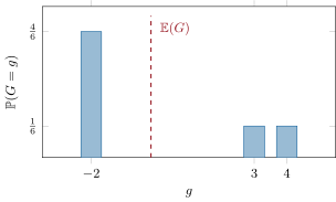
A game: pay $2$ euros, roll one fair die, receive the value shown if it is at least $5$ , nothing otherwise. Let $G$ be the gain (received minus paid). The outcomes $1, 2, 3, 4$ give $G = -2$ ; the outcome $5$ gives $G = 3$ ; the outcome $6$ gives $G = 4$ . The distribution of $G$ :

$g$	$-2$	$3$	$4$
$\P(G = g)$	$\dfrac46$	$\dfrac16$	$\dfrac16$

Method 18.7 (Building a distribution table)

List the possible values of $X$ ; for each value, collect the outcomes producing it and add their probabilities; check that the row of probabilities sums to $1$ .

18.3 Expectation

Definition 18.8 (Expectation)

The expectation (or mean) of $X$ is the average of its values weighted by their probabilities:

\E(X) = \sum_{i=1}^{k} \P(X = x_i)\; x_i .

Remark 18.9

$\E(X)$ is what the mean of a huge number of independent repetitions of the experiment would be — the precise version of this statement is the law of large numbers, proved in Chapter 34. Note the formal analogy with the mean of a dataset with frequencies (Definition 17.1): probabilities play the role of the relative frequencies $\frac{n_i}{n}$ .

Example 18.10

For the game of Example 18.6:

\E(G) = \frac46 \times (-2) + \frac16 \times 3 + \frac16 \times 4 = \frac{-8 + 3 + 4}{6} = -\frac16 \approx -0.17 .

On average the player loses about $17$ cents per game: the game is unfavorable. A game is called fair when the expected gain is $0$ .

Proposition 18.11 (Linearity)

For all reals $a, b$ :

\E(aX + b) = a\,\E(X) + b .

Proof. The variable $aX + b$ takes the value $a x_i + b$ with probability $\P(X = x_i)$ , so

\E(aX + b) = \sum_i \P(X = x_i)(a x_i + b) = a \sum_i \P(X = x_i)\,x_i + b \underbrace{\sum_i \P(X = x_i)}_{=\,1} = a\,\E(X) + b .

∎

18.4 Variance and standard deviation

Definition 18.12 (Variance)

The variance of $X$ measures the spread of its values around the expectation $m = \E(X)$ :

\V(X) = \E\bigl((X - m)^2\bigr) = \sum_{i=1}^{k} \P(X = x_i)\,(x_i - m)^2, \qquad \sigma(X) = \sqrt{\V(X)} .

Proposition 18.13 (Shortcut formula)

\V(X) = \E(X^2) - \E(X)^2 .

Proof. Expand $(x_i - m)^2 = x_i^2 - 2m\,x_i + m^2$ inside the sum:

\V(X) = \sum_i \P(X = x_i)\,x_i^2 - 2m \sum_i \P(X = x_i)\,x_i + m^2\sum_i \P(X = x_i) = \E(X^2) - 2m^2 + m^2 ,

which is $\E(X^2) - m^2$ . This is the random-variable version of the identity proved for datasets in Proposition 17.7. ∎

Proposition 18.14 (Affine transformation)

$\V(aX + b) = a^2\,\V(X)$ and $\sigma(aX + b) = \abs a\,\sigma(X)$ .

Proof. By linearity, $aX + b$ deviates from its expectation $a m + b$ by $(aX + b) - (am + b) = a(X - m)$ : every deviation is scaled by $a$ , hence every squared deviation by $a^2$ , and so is their weighted mean. The shift $b$ has disappeared — shifting a variable does not change its spread. ∎

Example 18.15

For the game of Example 18.6: $\E(G^2) = \frac46 \times 4 + \frac16 \times 9 + \frac16 \times 16 = \frac{16 + 9 + 16}{6} = \frac{41}{6}$ , so

\V(G) = \frac{41}{6} - \left(-\frac16\right)^2 = \frac{41}{6} - \frac{1}{36} = \frac{245}{36} \approx 6.8, \qquad \sigma(G) \approx 2.6 .

The loss of $0.17$ per game on average comes with swings of typical size $2.6$ euros — expectation without standard deviation tells only half the story.

The distribution of the gain G of , and its expectation (G) = -1/6 (dashed): the balance point of the probability masses. — The distribution of the gain $G$ of Example 18.6, and its expectation $\E(G) = -\frac16$ (dashed): the balance point of the probability masses.

18.5 Exercises

Exercise 18.1 ★

A card is drawn from a standard $52$ -card deck. Compute the probability of drawing: a heart; a king; a heart or a king; neither a heart nor a king.

Solution

Solution of Exercise 18.1.

Uniform model on $52$ cards. Hearts: $\frac{13}{52} = \frac14$ . Kings: $\frac{4}{52} = \frac{1}{13}$ . Heart or king: $\frac{13 + 4 - 1}{52} = \frac{16}{52} = \frac{4}{13}$ (the king of hearts is counted once). Neither: $1 - \frac{4}{13} = \frac{9}{13}$ .

Exercise 18.2 ★

Two fair dice are rolled and their sum $S$ is recorded. Using the $36$ -outcome model of Example 18.2, compute $\P(S = 6)$ , $\P(S \geq 10)$ and $\P(S \text{ is even})$ .

Solution

Solution of Exercise 18.2.

$S = 6$ : the pairs $(1,5), (2,4), (3,3), (4,2), (5,1)$ , so $\P(S = 6) = \frac{5}{36}$ .

$S \geq 10$ : three pairs for $10$ , two for $11$ , one for $12$ : $\P(S \geq 10) = \frac{6}{36} = \frac16$ .

$S$ even: sums $2, 4, 6, 8, 10, 12$ have $1 + 3 + 5 + 5 + 3 + 1 = 18$ pairs: probability $\frac{18}{36} = \frac12$ .

Exercise 18.3 ★

A random variable has distribution

$x$	$-1$	$0$	$2$	$5$
$\P(X=x)$	$0.3$	$0.2$	$0.4$	$p$

Find $p$ , then compute $\E(X)$ .

Solution

Solution of Exercise 18.3.

The probabilities sum to $1$ : $p = 1 - 0.3 - 0.2 - 0.4 = 0.1$ . Then

\E(X) = 0.3 \times (-1) + 0.2 \times 0 + 0.4 \times 2 + 0.1 \times 5 = -0.3 + 0.8 + 0.5 = 1 .

Exercise 18.4 ★

$X$ satisfies $\E(X) = 3$ and $\V(X) = 4$ . Give the expectation, variance and standard deviation of $Y = 2X - 5$ .

Solution

Solution of Exercise 18.4.

$\E(Y) = 2 \times 3 - 5 = 1$ ; $\V(Y) = 2^2 \times 4 = 16$ ; $\sigma(Y) = 4$ .

Exercise 18.5 ★★

A wheel of fortune has $10$ equal sectors: $5$ show $0$ euros, $3$ show $2$ euros, $2$ show $5$ euros. Playing costs $2$ euros. Give the distribution of the gain $G$ (winnings minus stake), compute $\E(G)$ , and decide whether the game is favorable.

Solution

Solution of Exercise 18.5.

The winnings are $0$ , $2$ , $5$ euros with probabilities $0.5$ , $0.3$ , $0.2$ ; subtracting the $2$ -euro stake, $G$ takes the values $-2, 0, 3$ :

$g$	$-2$	$0$	$3$
$\P(G=g)$	$0.5$	$0.3$	$0.2$

$\E(G) = -1 + 0 + 0.6 = -0.4$ : the player loses $40$ cents per game on average — unfavorable.

Exercise 18.6 ★★

An urn contains $3$ red and $2$ blue balls; two balls are drawn without replacement. Let $X$ be the number of red balls drawn. Build the distribution of $X$ (enumerate the $20$ ordered draws, or use a tree), and compute $\E(X)$ .

Solution

Solution of Exercise 18.6.

Drawing in order: $\P(X = 2) = \frac35 \times \frac24 = \frac{3}{10}$ (red then red); $\P(X = 0) = \frac25 \times \frac14 = \frac{1}{10}$ (blue then blue); hence $\P(X = 1) = 1 - \frac{3}{10} - \frac{1}{10} = \frac{6}{10}$ . Then

\E(X) = 0 \times \frac1{10} + 1 \times \frac6{10} + 2 \times \frac3{10} = \frac{12}{10} = 1.2 ,

consistent with intuition: $\frac35$ of the two draws are red on average.

Exercise 18.7 ★★

For the wheel of Exercise 18.5, compute $\V(G)$ and $\sigma(G)$ .

Solution

Solution of Exercise 18.7.

$\E(G^2) = 0.5 \times 4 + 0.3 \times 0 + 0.2 \times 9 = 3.8$ , so by the shortcut formula $\V(G) = 3.8 - (-0.4)^2 = 3.8 - 0.16 = 3.64$ and $\sigma(G) \approx 1.9$ euros.

Exercise 18.8 ★★

An insurance company sells a policy for $80$ euros. With probability $0.05$ the client claims $1000$ euros, with probability $0.01$ the client claims $5000$ euros, otherwise nothing. Let $B$ be the company’s benefit on one policy. Give the distribution of $B$ , compute $\E(B)$ , and interpret.

Solution

Solution of Exercise 18.8.

The benefit is $80$ minus the claim:

$b$	$80$	$-920$	$-4920$
$\P(B=b)$	$0.94$	$0.05$	$0.01$

$\E(B) = 75.2 - 46 - 49.2 = -20$ : at this price the company loses $20$ euros per policy on average. The premium is too low for the risks covered (it would need to exceed $100$ euros for a positive expected benefit).

Exercise 18.9 ★★

A multiple-choice question has $4$ answers, one correct. A correct answer scores $+1$ ; to discourage guessing, a wrong answer scores $x < 0$ . A student answers at random. For which value of $x$ is the student’s expected score zero?

Solution

Solution of Exercise 18.9.

The random score is $+1$ with probability $\frac14$ and $x$ with probability $\frac34$ :

\E = \frac14 + \frac{3x}{4} = 0 \iff x = -\frac13 .

With the penalty $-\frac13$ , random guessing brings nothing on average.

Exercise 18.10 ★★

Two fair coins are tossed. Ann proposes: “if both coins match, I pay you $1$ euro; if they differ, you pay me $1$ euro.” Compute the expected gain of each player. Is the game fair? Same question with three coins, where Ann pays $2$ euros if all three match.

Solution

Solution of Exercise 18.10.

Two coins: they match (HH or TT) with probability $\frac24 \times 2 = \frac12$ . The player’s gain is $+1$ or $-1$ with equal probabilities: expectation $0$ for both players — the game is fair.

Three coins: all match (HHH or TTT) with probability $\frac{2}{8} = \frac14$ . The player receives $2$ with probability $\frac14$ and pays $1$ with probability $\frac34$ : $\E = \frac24 - \frac34 = -\frac14$ . The game favours Ann by $25$ cents per round; it would be fair if she paid $3$ euros for a triple match.

Exercise 18.11 ★★★

A lottery sells $1000$ tickets at $5$ euros each. One ticket wins $2000$ euros, five tickets win $200$ euros, twenty tickets win $25$ euros.

Give the distribution of the organizer’s total revenue minus prizes, and of a single player’s gain $G$ .
Compute $\E(G)$ and the total expected profit of the organizer. Check that the two answers are consistent.

Solution

Solution of Exercise 18.11.

1. The organizer receives $1000 \times 5 = 5000$ euros and pays out $2000 + 5 \times 200 + 20 \times 25 = 3500$ euros in all: the profit is the constant $1500$ (no randomness once all tickets are sold). A single player’s gain $G$ (prize minus the $5$ -euro ticket):

$g$	$1995$	$195$	$20$	$-5$
$\P(G=g)$	$\dfrac{1}{1000}$	$\dfrac{5}{1000}$	$\dfrac{20}{1000}$	$\dfrac{974}{1000}$

\E(G) = \frac{1995 + 5 \times 195 + 20 \times 20 - 974 \times 5}{1000} = \frac{1995 + 975 + 400 - 4870}{1000} = -1.5 .

Each player expects to lose $1.50$ euros; over $1000$ players that is $1500$ euros — exactly the organizer’s profit. The books balance: what the players lose on average is precisely what the organizer collects.

18.6 Problem: The unfinished game

Problem 18.1

Weekend problem — Pascal, Fermat and the fair split of an interrupted bet: the birth of expectation, the magic of linearity, and what expectation cannot see

In 1654 the Chevalier de Méré — the same gambler whose dice bets opened the Middle School volume’s probability problem — asked Blaise Pascal a deeper question: two equally skilled players must stop their series at the score of $5$ to $3$ , six wins taking the $64$ -pistole pot. How should the pot be split fairly? The letters between Pascal and Fermat answering it founded the concept at the heart of this chapter: expectation (Definition 18.8). You will re-derive their answer both ways, then meet linearity’s party trick and expectation’s one blind spot.

Part I — Expectation fluency.

Roll a fair die; your gain is (face $- 3$ ) euros. Build the distribution table of the gain $G$ (Method 18.7) and compute $\E(G)$ .
Compute $V(G)$ with the shortcut formula (Proposition 18.13) and $\sigma(G)$ (two decimals).
Without any new table, give $\E(2G - 1)$ and $V(2G - 1)$ (Proposition 18.14).
A stall charges $m$ euros to roll two dice and pockets you the sum in euros. What is the fair price $m$ ? The stall charges $8$ : what is your expected loss per game?
A laptop worth $800$ euros has a $5\,\%$ chance of destruction each year. Compute the fair insurance premium, and the insurer’s expected profit per policy if it charges $60$ euros.

Part II — Splitting the pot. Score $5$ – $3$ , first to $6$ wins the $64$ pistoles, rounds are fair coin flips.

Two tempting wrong answers: split $5 : 3$ (proportionally to rounds won), or give everything to the leader. Say in one sentence each what is unfair about them.
Fermat’s method: player A needs $1$ more win, B needs $3$ ; imagine playing exactly $3$ more rounds regardless. List the $8$ equally likely outcomes, mark who wins the series in each, and deduce the fair split of the $64$ pistoles.
The subtle point Fermat had to defend: the real game might stop after one round — why is it nevertheless legitimate to reason on all $3$ imaginary rounds?
Pascal’s method, backwards from the end: compute A’s fair share at the (hypothetical) scores $5$ – $5$ , then $5$ – $4$ , then $5$ – $3$ , each time averaging the two equally likely futures. Compare with question 7.
Same question at the score $4$ – $3$ : how many imaginary rounds, which outcomes give B the series, and what is the fair split?
State the principle the two methods share — the fair value of an uncertain future is its expectation — and name two modern industries running entirely on it (question 5 shows one).
A sanity check for every score: explain, with the linearity of expectation (Proposition 18.11), why the two players’ fair shares must always add up to exactly the $64$ -pistole pot.

Part III — Linearity’s party trick.

Recover $\E(\text{sum of two dice}) = 7$ in one line with linearity (Proposition 18.11), no $36$ -cell table. For the variance of the sum, the rule $V(X + Y) = V(X) + V(Y)$ needs the dice to be independent (admitted): compute it.
The hat-check party: $n$ guests throw their hats in a pile and each takes one back at random. Let $X$ count the guests who recover their own hat. For one fixed guest, what is the probability of recovering their own hat? Summing these $n$ chances (linearity!), compute $\E(X)$ . The answer should surprise you: it does not depend on $n$ .
Verify $\E(X) = 1$ by brute force for $n = 2$ and $n = 3$ (list the $2$ and $6$ equally likely hat-assignments and average the counts).
The guests’ recoveries are far from independent (if $n - 1$ guests got their own hats back, the last one must too). Where exactly did question 14’s computation not require independence? State linearity’s superpower.

Part IV — What expectation cannot see.

Two $5$ -euro scratch cards: card A wins $10$ euros with probability $\frac12$ ; card B wins $1\,000$ euros with probability $0.005$ . Check that both gains have the same expectation, then compute both variances. Which card do real people buy, and what are they buying?
The St Petersburg game: flip until the first tails; if the first tails occurs at flip $n$ you receive $2^n$ euros. Compute the contribution of each $n$ to the expectation and the expectation itself. Would you pay $1\,000$ euros to play once? What does the clash teach about expectation?
Insurance from the customer’s side: pay $20$ euros, or face a $1\,\%$ risk of losing $1\,000$ ? Compare the two expectations, and explain why buying the insurance can still be rational (what can a single family not “average over”?).
Finale — expectation’s biography, one sentence per chapter: born in 1654 to split a pot; its superpower, linearity, which adds expectations without asking independence (the hats); its blind spot, risk, which variance measures (cards, St Petersburg, insurance); and its coronation next year, when the law of large numbers explains exactly why the house always wins.

Solution

Solution of Problem 18.1.

1. $G$ takes $-2, -1, 0, 1, 2, 3$ , each with probability $\frac16$ : $\E(G) = \frac{-2 - 1 + 0 + 1 + 2 + 3}{6} = \frac12$ euro.

2. $\E(G^2) = \frac{4 + 1 + 0 + 1 + 4 + 9}{6} = \frac{19}{6}$ ; $V(G) = \frac{19}{6} - \frac14 = \frac{35}{12} \approx 2.92$ ; $\sigma(G) \approx 1.71$ .

3. $\E(2G - 1) = 2 \times \frac12 - 1 = 0$ ; $V(2G - 1) = 4\,V(G) = \frac{35}{3}$ .

4. $\E(\text{sum}) = 7$ : fair price $7$ euros. At $8$ , the expected loss is $1$ euro per game.

5. Fair premium: $0.05 \times 800 = 40$ euros. Charging $60$ : expected profit $20$ euros per policy.

6. Splitting $5:3$ rewards the past — but the pot belongs to whoever wins the future, and B might still win. Giving all to A treats a probable win as certain — B’s small chance is worth something.

7. Rounds to play: $3$ ; outcomes (A-win/B-win per round): AAA, AAB, ABA, ABB, BAA, BAB, BBA, BBB. Player B takes the series only by winning all three: BBB alone. A wins the series in $7$ of $8$ cases: fair split $64 \times \frac78 = 56$ pistoles for A, $8$ for B.

8. Playing the extra, pointless rounds changes nobody’s victory: once A has her sixth win, later rounds are ceremony. But fixing the horizon at exactly $3$ rounds makes all $8$ outcomes equally likely — honest counting needs same-length stories, and padding them out costs nothing.

9. At $5$ – $5$ : one deciding round, $32$ each. At $5$ – $4$ : A gets $\frac{64 + 32}{2} = 48$ . At $5$ – $3$ : the next round leads to $64$ (A wins it) or to the $5$ – $4$ position worth $48$ : A’s share $\frac{64 + 48}{2} = 56$ — Fermat’s $56 : 8$ , re-derived by walking backwards.

10. A needs $2$ , B needs $3$ : play $4$ imaginary rounds ( $16$ outcomes). B takes the series with $3$ or $4$ B-wins: $4 + 1 = 5$ outcomes. Split: $B$ : $64 \times \frac{5}{16} = 20$ ; $A$ : $44$ .

11. The fair present value of an uncertain future payoff is its expectation — probability-weighted average of what may come. Insurance (question 5) and finance (pricing uncertain payoffs) are this sentence turned into industries; so are casinos, from the other side of the table.

12. The pot always ends up somewhere: the two shares are random variables summing to the constant $64$ , so by linearity $\E_A + \E_B = 64$ — fair shares exhaust the pot, at every score.

13. Linearity: $\E(X + Y) = 3.5 + 3.5 = 7$ , table-free — true even for glued-together dice. Variance of one die: $\E(X^2) - 3.5^2 = \frac{91}{6} - \frac{49}{4} = \frac{35}{12}$ ; for independent dice $V(X + Y) = \frac{35}{12} + \frac{35}{12} = \frac{35}{6}$ .

14. Each fixed guest recovers their own hat with probability $\frac1n$ (their hat is one among $n$ ). Summing over the $n$ guests: $\E(X) = n \times \frac1n = 1$ — one lucky guest on average, whether the party has two hats or two thousand.

15. $n = 2$ : assignments: both right ( $X = 2$ ) or swapped ( $X = 0$ ): $\E = 1$ . $n = 3$ : the six assignments give $X = 3, 1, 1, 1, 0, 0$ : $\E = \frac{6}{6} = 1$ .

16. The computation added the expectations of the $n$ individual indicators (“guest $i$ got their hat”), and linearity adds expectations unconditionally — dependence would wreck a product or a variance, but never a sum of expectations. That is linearity’s superpower: no independence questions asked.

17. Both gains: $\E = 0.5 \times 10 - 5 = 0$ and $0.005 \times 1000 - 5 = 0$ . Variances (of the gain): A: $\E(G^2) = 0.5 \times 25 + 0.5 \times 25 = 25$ ; B: $0.005 \times 995^2 + 0.995 \times 25 \approx 4\,975$ : $\sigma_A = 5$ , $\sigma_B \approx 70.5$ . People buy B: what they purchase is not expectation (zero in both) but the spread — a small chance of a life-changing right tail.

18. First tails at flip $n$ has probability $2^{-n}$ and pays $2^n$ : each $n$ contributes $2^{-n} \times 2^n = 1$ to the expectation, which is therefore $1 + 1 + 1 + \dots$ : infinite. Yet no sane person pays $1\,000$ to play once: with probability $\frac{15}{16}$ the payout is at most $16$ . Expectation summarizes the long run of repeatable bets; a once-in-a-lifetime game with a wild tail is not priced by its mean.

19. Expectations: insure $-20$ ; go bare $-0.01 \times 1000 = -10$ . The naked strategy wins on average — for someone who can absorb the loss and repeat the bet many times. A family that cannot survive the $-1\,000$ is not in the averaging business: it pays $10$ extra to delete the variance. Insurers average; households buy certainty.

20. Born splitting a pot between two impatient gamblers; empowered by linearity, which sums hopes without asking permission of dependence; blind to risk, which variance — the lotteries, the Petersburg game, the family’s policy — must measure instead; and crowned next year by the law of large numbers, which explains why the averages always, eventually, collect.