High School Mathematics · Grades 10–12

34Sums of Random Variables and the Law of Large Numbers

Why do casinos always win in the end, and why do polls work? Because averages of many independent random quantities fluctuate less and less. This chapter proves it: linearity of expectation, additivity of variance for independent variables, the Bienaymé–Chebyshev inequality, and the law of large numbers.

34.1 Sums of random variables

Given two random variables $X, Y$ on the same finite sample space $\Omega$ , the sum $X + Y$ is the random variable $\omega \mapsto X(\omega) + Y(\omega)$ .

Theorem 34.1 (Linearity of expectation)

For all random variables $X, Y$ on $\Omega$ and $a, b \in \R$ :

\E(X + Y) = \E(X) + \E(Y), \qquad \E(aX + b) = a\E(X) + b .

No independence assumption is needed.

Proof. Write the expectation as a sum over outcomes: since $\P(X = x) = \sum_{\omega : X(\omega) = x} \P(\{\omega\})$ , grouping terms gives $\E(X) = \sum_{\omega \in \Omega} \P(\{\omega\})\,X(\omega)$ . Then

\E(X + Y) = \sum_{\omega} \P(\{\omega\})\bigl(X(\omega) + Y(\omega)\bigr) = \sum_{\omega} \P(\{\omega\})X(\omega) + \sum_{\omega} \P(\{\omega\})Y(\omega) = \E(X) + \E(Y). \qedhere

∎

Definition 34.2 (Independent random variables)

$X$ and $Y$ are independent if for all values $x, y$ :

\P(X = x \text{ and } Y = y) = \P(X = x)\,\P(Y = y).

Several variables $X_1, \dots, X_n$ are independent if this product rule holds for every choice of values of every subfamily.

Proposition 34.3

If $X$ and $Y$ are independent, $\E(XY) = \E(X)\,\E(Y)$ .

Proof.

\begin{aligned} \E(XY) &= \sum_{x, y} xy\;\P(X = x \text{ and } Y = y) = \sum_{x, y} xy\,\P(X=x)\P(Y=y) \\ &= \Bigl(\sum_x x\P(X=x)\Bigr)\Bigl(\sum_y y\P(Y=y)\Bigr). \qedhere \end{aligned}

∎

Theorem 34.4 (Variance of a sum)

If $X$ and $Y$ are independent, then

\V(X + Y) = \V(X) + \V(Y).

More generally, for independent $X_1, \dots, X_n$ : $\V(X_1 + \dots + X_n) = \V(X_1) + \dots + \V(X_n)$ .

Proof. Using König–Huygens (Proposition 33.3) and linearity:

\begin{align*} \V(X + Y) &= \E\bigl((X+Y)^2\bigr) - \bigl(\E X + \E Y\bigr)^2\\ &= \E(X^2) + 2\E(XY) + \E(Y^2) - \E(X)^2 - 2\E(X)\E(Y) - \E(Y)^2\\ &= \V(X) + \V(Y) + 2\bigl(\E(XY) - \E(X)\E(Y)\bigr), \end{align*}

and the last bracket vanishes for independent variables (Proposition 34.3). The general case follows by induction. ∎

Example 34.5 (Binomial revisited)

A binomial variable $X \sim \mathcal B(n, p)$ is a sum $X = X_1 + \dots + X_n$ of $n$ independent Bernoulli variables. Hence, structurally:

\E(X) = np, \qquad \V(X) = np(1-p),

recovering Theorem 33.8 without any computation.

Proposition 34.6 (Sample mean)

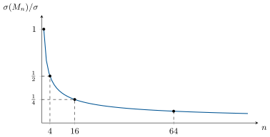
Let $X_1, \dots, X_n$ be independent with the same distribution as $X$ (expectation $\mu$ , variance $\sigma^2$ ), and let $M_n = \frac{X_1 + \dots + X_n}{n}$ be their sample mean. Then

\E(M_n) = \mu, \qquad \V(M_n) = \frac{\sigma^2}{n}, \qquad \sigma(M_n) = \frac{\sigma}{\sqrt n}.

Proof. Linearity gives $\E(M_n) = \frac{n\mu}{n} = \mu$ ; independence gives $\V(X_1 + \dots + X_n) = n\sigma^2$ , and dividing by $n$ scales the variance by $\frac{1}{n^2}$ (Proposition 33.4). ∎

The $\frac{\sigma}{\sqrt n}$ is the fundamental square root law: to halve the fluctuations of an average, quadruple the sample size.

The square root law: each quadrupling of the sample size only halves the standard deviation of the mean.

34.2 Concentration inequalities

Theorem 34.7 (Markov’s inequality)

If $X \geq 0$ and $a > 0$ :

\P(X \geq a) \leq \frac{\E(X)}{a}.

Proof. In $\E(X) = \sum_i p_i x_i$ (all terms nonnegative), keep only the terms with $x_i \geq a$ : each is at least $a\,p_i$ , so $\E(X) \geq a \sum_{x_i \geq a} p_i = a\,\P(X \geq a)$ . ∎

Theorem 34.8 (Bienaymé–Chebyshev inequality)

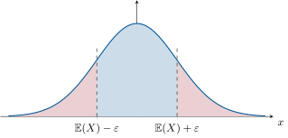
For any random variable $X$ and any $\varepsilon > 0$ :

\P\bigl(\abs{X - \E(X)} \geq \varepsilon\bigr) \leq \frac{\V(X)}{\varepsilon^2}.

Proof. Apply Markov’s inequality to the nonnegative variable $Y = (X - \E(X))^2$ with $a = \varepsilon^2$ :

\P\bigl(\abs{X - \E(X)} \geq \varepsilon\bigr) = \P(Y \geq \varepsilon^2) \leq \frac{\E(Y)}{\varepsilon^2} = \frac{\V(X)}{\varepsilon^2}. \qedhere

∎

Concentration: Bienaymé–Chebyshev bounds the probability that X falls in the tails (red), at distance at least from its expectation, by (X)/ 2. — Concentration: Bienaymé–Chebyshev bounds the probability that $X$ falls in the tails (red), at distance at least $\varepsilon$ from its expectation, by $\V(X)/\varepsilon^2$ .

Theorem 34.9 (Law of large numbers)

Let $X_1, \dots, X_n$ be independent with the same distribution (expectation $\mu$ , variance $\sigma^2$ ) and $M_n$ their sample mean. For every $\varepsilon > 0$ :

\P\bigl(\abs{M_n - \mu} \geq \varepsilon\bigr) \leq \frac{\sigma^2}{n\,\varepsilon^2} \xrightarrow[n \to +\infty]{} 0 .

The sample mean concentrates around the expectation.

Proof. Bienaymé–Chebyshev applied to $M_n$ , whose expectation is $\mu$ and whose variance is $\frac{\sigma^2}{n}$ (Proposition 34.6). ∎

Remark 34.10

This theorem is the bridge between probability theory and statistics: the frequency of an event over many independent repetitions approaches its probability (take $X_i$ the indicator of the event, so that $\mu = p$ ). It justifies estimating a probability by simulation (Monte Carlo method) and a population proportion by a poll — quantitatively: see Chapter 35.

Method 34.11 (Using Bienaymé–Chebyshev)

To guarantee $\P(\abs{M_n - \mu} \geq \varepsilon) \leq \alpha$ , it suffices that $n \geq \frac{\sigma^2}{\alpha\,\varepsilon^2}$ . The bound is crude (real fluctuations are usually much smaller) but perfectly general: it requires nothing about the distribution beyond a finite variance.

34.3 Exercises

Exercise 34.1 ★

Two fair dice are rolled; let $S$ be the sum. Using linearity (not the distribution of $S$ !), compute $\E(S)$ ; then compute $\V(S)$ using independence, given that a single fair die has variance $\frac{35}{12}$ .

Solution

Solution of Exercise 34.1.

Each die has expectation $\frac{1 + 2 + \dots + 6}{6} = \frac{7}{2}$ , so by linearity $\E(S) = \frac72 + \frac72 = 7$ . The dice are independent, so $\V(S) = \frac{35}{12} + \frac{35}{12} = \frac{35}{6} \approx 5.83$ .

Exercise 34.2 ★

Let $X \sim \mathcal B(100,\ 0.5)$ . Bound $\P(X \geq 75)$ using Markov’s inequality, then $\P(\abs{X - 50} \geq 25)$ using Bienaymé–Chebyshev. Compare.

Solution

Solution of Exercise 34.2.

$\E(X) = 50$ and $\V(X) = 100 \times 0.25 = 25$ .

Markov ( $X \geq 0$ ): $\P(X \geq 75) \leq \frac{50}{75} = \frac23$ .

Bienaymé–Chebyshev: $\P(\abs{X - 50} \geq 25) \leq \frac{25}{25^2} = 0.04$ — and this even bounds the two-sided event, of which $X \geq 75$ is half. Chebyshev is far sharper here because it exploits the variance, not just the mean. (The true value of $\P(X \geq 75)$ is smaller than $10^{-6}$ : both bounds are crude.)

Exercise 34.3 ★

A fair coin is tossed $n$ times and $F_n$ denotes the frequency of heads. How large must $n$ be so that, by the Bienaymé–Chebyshev bound, $\P\bigl(\abs{F_n - 0.5} \geq 0.05\bigr) \leq 0.05$ ?

Solution

Solution of Exercise 34.3.

$F_n$ is the sample mean of $n$ Bernoulli $\left(\frac12\right)$ variables, of variance $\sigma^2 = \frac14$ . The bound

\P\left(\abs{F_n - 0.5} \geq 0.05\right) \leq \frac{1/4}{n \times 0.05^2} = \frac{100}{n}

is $\leq 0.05$ as soon as $n \geq 2000$ .

Exercise 34.4 ★★

An investor splits her capital equally between $n$ independent assets, each with expected return $\mu = 5\%$ and standard deviation $\sigma = 20\%$ . Compute the expectation and standard deviation of the portfolio return $M_n$ , and the number of assets needed to bring the standard deviation below $4\%$ . What financial principle does this illustrate?

Solution

Solution of Exercise 34.4.

By Proposition 34.6, $\E(M_n) = 5\%$ (diversification does not change the expected return) and $\sigma(M_n) = \frac{20\%}{\sqrt n}$ . Requiring $\frac{20}{\sqrt n} < 4$ gives $\sqrt n > 5$ , i.e. $n \geq 26$ . This is the principle of diversification: spreading capital over independent risks divides the risk (standard deviation) by $\sqrt n$ without reducing the expected return.

Exercise 34.5 ★★

Let $X$ and $Y$ be independent, both uniform on $\{1, 2, 3\}$ .

Give the distribution of $S = X + Y$ and compute $\E(S)$ , $\V(S)$ directly from it.
Recover both values by linearity and additivity of variance.

Solution

Solution of Exercise 34.5.

1. Counting the $9$ equally likely pairs: $S$ takes the values $2, 3, 4, 5, 6$ with probabilities $\frac19, \frac29, \frac39, \frac29, \frac19$ . Hence $\E(S) = \frac{2 + 6 + 12 + 10 + 6}{9} = 4$ and $\E(S^2) = \frac{4 + 18 + 48 + 50 + 36}{9} = \frac{156}{9} = \frac{52}{3}$ , so $\V(S) = \frac{52}{3} - 16 = \frac43$ .

2. One variable: $\E(X) = 2$ , $\E(X^2) = \frac{1 + 4 + 9}{3} = \frac{14}{3}$ , $\V(X) = \frac{14}{3} - 4 = \frac23$ . Then $\E(S) = 2 + 2 = 4$ and, by independence, $\V(S) = \frac23 + \frac23 = \frac43$ . Same values.

Exercise 34.6 ★★

Show that the additivity of variance can fail without independence: compute $\V(X + Y)$ for $Y = X$ , and compare with $\V(X) + \V(Y)$ . For which variables $X$ is $\V(2X) = 2\V(X)$ ?

Solution

Solution of Exercise 34.6.

With $Y = X$ : $\V(X + Y) = \V(2X) = 4\V(X)$ , while $\V(X) + \V(Y) = 2\V(X)$ . The two agree only when $\V(X) = 0$ , i.e. when $X$ is constant — so additivity genuinely requires independence (here $X$ is maximally dependent on itself).

Exercise 34.7 ★★

A die is suspected of being loaded. It is rolled $1200$ times and shows a six $260$ times ( $f = 0.2167$ instead of $\frac16 \approx 0.1667$ ). Under the hypothesis that the die is fair, bound $\P\bigl(\abs{F_n - \frac16} \geq 0.05\bigr)$ by Bienaymé–Chebyshev, and discuss whether the fairness hypothesis is plausible.

Solution

Solution of Exercise 34.7.

Under fairness, $F_n$ is the mean of $n = 1200$ Bernoulli variables with $p = \frac16$ , $\sigma^2 = \frac16\cdot\frac56 = \frac{5}{36}$ :

\P\left(\abs{F_n - \tfrac16} \geq 0.05\right) \leq \frac{5/36}{1200 \times 0.0025} = \frac{5}{108} \approx 0.046 .

The observed deviation is exactly $0.05$ : an event that a fair die produces with probability at most $4.6\%$ — and since Chebyshev is very conservative, the true probability is far smaller. The fairness hypothesis is not plausible; the die is very likely loaded.

Exercise 34.8 ★★★

(A better inequality for the coin.) Let $X \sim \mathcal B(n,\ p)$ and $F_n = \frac Xn$ .

Show that $p(1-p) \leq \frac14$ for $p \in \intcc{0}{1}$ .
Deduce the distribution-free bound $\P\bigl(\abs{F_n - p} \geq \varepsilon\bigr) \leq \frac{1}{4n\varepsilon^2}$ .
How many people must be polled so that the observed frequency is within $3$ points of the true proportion with probability at least $95\%$ , using this bound? (Real polls use sharper estimates, but the order of magnitude is right.)

Solution

Solution of Exercise 34.8.

1. $p(1-p) = \frac14 - \left(p - \frac12\right)^2 \leq \frac14$ .

2. $F_n$ has expectation $p$ and variance $\frac{p(1-p)}{n} \leq \frac{1}{4n}$ ; Bienaymé–Chebyshev gives

\P\bigl(\abs{F_n - p} \geq \varepsilon\bigr) \leq \frac{p(1-p)}{n\varepsilon^2} \leq \frac{1}{4n\varepsilon^2},

valid whatever the unknown $p$ .

3. With $\varepsilon = 0.03$ and level $0.05$ :

\frac{1}{4n(0.03)^2} \leq 0.05 \iff n \geq \frac{1}{4 \times 0.0009 \times 0.05} \approx 5556 .

About $5600$ people suffice by this crude bound (the classical normal-approximation answer is nearer $1100$ , see Chapter 35).

34.4 Problem: The house always wins

Problem 34.1

Weekend problem — the law of large numbers explains casinos, polls and insurance, and demolishes the gambler’s fallacy on the way

A roulette player after $100$ spins is, almost as often as not, ahead. The casino running a million spins is ahead with a certainty no court would question. Same game, same tiny edge — the difference is $\sqrt n$ , and it is the subject of this chapter (Proposition 34.6, Theorem 34.8, Theorem 34.9). This problem runs the casino’s books, sizes an election poll, prices diversification — and dismantles the most expensive fallacy in the history of gambling.

Part I — Fluency.

Two independent dice: compute $V(X + Y)$ (Theorem 34.4).
Roll $100$ independent dice and average the results: give the expectation and the standard deviation of the sample mean (Proposition 34.6; for one die, $\sigma = \sqrt{35/12} \approx 1.71$ ).
A nonnegative random variable has expectation $2$ . What does Markov’s inequality (Theorem 34.7) say about $\P(X \geq 10)$ ?
Bound $\P\left(\abs{\bar X_{100} - 3.5} \geq 0.5\right)$ for the dice average of question 2 with Bienaymé–Chebyshev.
Expectations add always, variances only under independence: exhibit dependent $X, Y$ (hint: $Y = -X$ ) for which $V(X + Y) \neq V(X) + V(Y)$ .

Part II — The house’s books. European roulette, bet $1$ euro on red: win $+1$ with probability $\frac{18}{37}$ , lose $-1$ with probability $\frac{19}{37}$ .

Compute the expectation and standard deviation of one bet’s gain.
A gambler makes $100$ independent bets; let $G$ be the total gain. Compute $\E(G)$ and $\sigma(G)$ , then the ratio $\frac{\abs{\E(G)}}{\sigma(G)}$ . What does a drift of a quarter of a standard deviation mean for the gambler’s chances of being ahead tonight?
The casino sees $1\,000\,000$ bets. Compute the expectation and standard deviation of its total take, and the same ratio. Interpret the number $27$ .
Certify with Chebyshev: bound the probability that the casino loses money over the million bets.
Betting systems: doubling after losses, quitting when ahead … Using the linearity of expectation (Theorem 34.1) over the (possibly random) sequence of stakes, explain why every strategy in a negative-edge game has negative expected gain — what would a winning system violate?
State what the law of large numbers (Theorem 34.9) promises about the frequency of red — and what it does not promise about the next spin after ten reds in a row. Name the fallacy.
The subtlest point: the law works by dilution, not compensation. If reds run $100$ ahead of expectation after some evening, the surplus is never “paid back” — compute what happens instead to the fraction $\frac{100}{n}$ by $n = 10^6$ , and rewrite the gambler’s fallacy’s error in one sentence.

Part III — Polls.

From Exercise 34.8: how many people must be polled for the observed frequency to fall within $3$ points of the truth with probability at least $95\,\%$ , by the distribution-free Chebyshev bound?
Real polling institutes use about $1\,100$ people for a $\pm 3$ -point margin at $95\,\%$ : their formula is $n \approx \frac{1.96^2 \times p(1-p)} {\varepsilon^2}$ with $p(1-p) \leq \frac14$ . Evaluate it, and explain the gap with question 13 (what does Chebyshev not know about the shape of the fluctuations?).
To halve the margin of error, how must the sample grow? From $\pm 3$ points at $1\,100$ , what sample gives $\pm 1.5$ points?
The counterintuitive classic: the required sample size never used the population’s size — $1\,100$ people suffice for a city or a continent. Point to the place in the model where the population size is absent, and give the kitchen analogy that pollsters use.

Part IV — Diversification.

The insurer of Problem 33.1 earns $30n$ euros in expectation on $n$ policies with a claims standard deviation of about $315\sqrt n$ . For which $n$ does the expected profit finally exceed one standard deviation of the claims? What is the $\sqrt n$ doing for the insurer?
One stock’s yearly return fluctuates with $\sigma = 20\,\%$ . Split the money equally over $25$ independent such stocks: compute the portfolio’s $\sigma$ . Finance calls diversification the only free lunch — what is the lunch, exactly?
Now let the $25$ stocks be perfectly correlated (they all move together): what is the portfolio’s $\sigma$ ? Compare the two extremes and state which assumption every diversification argument secretly rents — and what happened when it failed system-wide in 2008.
Finale — the $\sqrt n$ symphony: sums fluctuate like $\sqrt n$ while their means settle like $\frac{1}{\sqrt n}$ ; play the theme through the four industries of this problem (casino, polling, insurance, portfolios), name the two standing abusers (the gambler’s fallacy and fake independence), and give the forward pointer: the shape of the fluctuations — the bell — is the next chapter’s continuous star, and its full theorem crowns the university volumes.

Solution

Solution of Problem 34.1.

1. $V(X + Y) = V(X) + V(Y) = \frac{35}{12} + \frac{35}{12} = \frac{35}{6}$ (independence).

2. $\E(\bar X) = 3.5$ ; $\sigma(\bar X) = \frac{1.71}{\sqrt{100}} \approx 0.17$ : the hundred-dice average hugs $3.5$ within a fifth of a point.

3. $\P(X \geq 10) \leq \frac{2}{10} = 0.2$ .

4. $\P \leq \frac{V(\bar X)}{0.5^2} = \frac{35/1200}{0.25} \approx 0.117$ : at most about $12\,\%$ .

5. With $Y = -X$ : $V(X + Y) = V(0) = 0$ , while $V(X) + V(Y) = 2V(X) > 0$ : perfectly anti-correlated variables cancel — variance addition is an independence privilege.

6. $\E = \frac{18}{37} - \frac{19}{37} = -\frac{1}{37} \approx -0.027$ ; $\sigma = \sqrt{1 - \left(\frac{1}{37}\right)^2} \approx 1.00$ .

7. $\E(G) = -2.70$ , $\sigma(G) = 10 \times 1.00 = 10$ : the drift is only $0.27\sigma$ . The night’s noise dwarfs the edge — a large minority of gamblers (roughly $40\,\%$ , says the bell) walk out ahead, which is precisely what keeps them coming back.

8. Casino’s take: expectation $+27\,027$ euros, standard deviation $\approx 1\,000$ : the profit sits $27$ standard deviations above zero. At $27\sigma$ , “the casino might lose this year” is not a risk, it is a rounding error.

9. $\P(\text{loss}) = \P(G \geq 27\,027$ for the gamblers $)$ $\leq \frac{10^6 \times 1}{27\,027^2} \approx 0.0014$ : even the bluntest inequality in the book guarantees the house at $99.86\,\%$ — the truth is astronomically stronger.

10. Each euro staked, whenever and however chosen, has expected return $-\frac{1}{37}$ of itself; by linearity the expected total gain is $-\frac{1}{37} \times (\text{total staked})$ , negative for every strategy that stakes anything. A winning system would violate the linearity of expectation — no clever sequencing of bad bets makes a good one. (Doubling systems merely trade many small wins for rare catastrophic losses.)

11. The theorem: the frequency of red over $n$ spins converges (in probability) to $\frac{18}{37}$ . It says nothing about spin $n + 1$ : the wheel has no memory, and after ten reds the chance of red is still $\frac{18}{37}$ . Believing otherwise is the gambler’s fallacy, and question 12 shows what actually happens to streaks.

12. The surplus of $100$ reds is not repaid — future spins are fair copies, expected surplus stays $100$ . But $\frac{100}{10^6} = 0.0001$ : one hundredth of a point. The fallacy’s error in one sentence: the law of large numbers dilutes past accidents in an ocean of new trials; it never sends the wheel to collect debts.

13. $n \geq \frac{1}{4 \times 0.05 \times 0.03^2} \approx 5\,556$ people.

14. $\frac{1.96^2 \times 0.25}{0.03^2} \approx 1\,067$ : five times fewer. Chebyshev holds for every distribution and pays for its universality with slack; the pollsters’ constant $1.96$ comes from the actual bell shape of the fluctuations, which concentrates far harder.

15. Margin $\propto \frac{1}{\sqrt n}$ : halving it quadruples the sample — about $4\,400$ people for $\pm 1.5$ points. Precision is bought at quadratic prices.

16. The model is $n$ independent draws with success probability $p$ — the population size $N$ never appears (sampling a tiny fraction of a large, well-mixed population is what independence encodes). The pollsters’ analogy: to taste the soup, one well-stirred spoonful suffices — whether the pot serves ten or ten thousand. The catch is the stirring — a biased sampling frame, as in the Middle School volume’s poll that fooled a country — not the pot.

17. $315\sqrt n < 30n \iff \sqrt n > 10.5 \iff n > 110$ : beyond a hundred policies the drift outruns the noise, and each further policy widens the gap by the $\sqrt n$ law — pooling is the business model.

18. Independent equal shares: $\sigma_{\text{pf}} = \frac{20\,\%}{\sqrt{25}} = 4\,\%$ : same expected return, one-fifth the fluctuation. The lunch: risk reduction at zero cost in expectation — averaging independent randomness.

19. Perfectly correlated: the portfolio is one stock in $25$ costumes: $\sigma = 20\,\%$ , no reduction at all. Diversification rents independence; when a crisis correlates everything (2008: all housing bets were one bet), the $\sqrt n$ protection evaporates exactly when it is needed.

20. Sums drift like $n$ and fluctuate like $\sqrt n$ , so means settle like $\frac{1}{\sqrt n}$ : the casino banks the drift over a million spins; the pollster buys $\frac{1}{\sqrt{1100}}$ of noise for a phone budget; the insurer outgrows its own claims at $n > 110$ ; the investor divides risk by $\sqrt{25}$ . Abusers: the gambler who believes in debts (there is only dilution), and the financier who believes in independence (there is sometimes only one bet). The fluctuations’ universal shape — the bell — is the continuous chapter’s star, and its theorem, the central limit theorem, is the summit of the university volumes’ probability.