High School Mathematics · Grades 10–12

17Descriptive Statistics

Statistics compresses a list of numbers into a few meaningful summaries: where the data sits (mean, median), and how spread out it is (quartiles, variance, standard deviation). This chapter works everything out on one running example. The same summaries reappear for random variables in Chapter 18, and their probabilistic laws in Chapter 34.

Throughout the chapter, our running dataset is the marks (out of $20$ ) of a class of $12$ students:

8,\ 9,\ 10,\ 10,\ 11,\ 12,\ 12,\ 12,\ 13,\ 14,\ 16,\ 17 .

17.1 Mean and median

Definition 17.1 (Mean)

The mean of the values $x_1, x_2, \dots, x_n$ is

\bar x = \frac{x_1 + x_2 + \dots + x_n}{n}.

If the value $x_i$ appears with frequency $n_i$ (with $n_1 + \dots + n_k = n$ ), then $\bar x = \frac{n_1 x_1 + \dots + n_k x_k}{n}$ .

Definition 17.2 (Median)

A median of a sorted dataset is a value that splits it in half: at least half the values are $\leq$ it, and at least half are $\geq$ it. In practice, sort the $n$ values; if $n$ is odd, the median is the middle value; if $n$ is even, take the midpoint of the two middle values.

Example 17.3

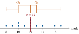
For the running dataset, the sum is $144$ , so $\bar x = \frac{144}{12} = 12$ . The two middle values ( $6$ th and $7$ th of the sorted list) are both $12$ , so the median is $12$ too. Mean and median need not coincide: the median ignores how far the extreme values are, the mean does not. Replacing the top mark $17$ by $20$ moves the mean to $12.25$ but leaves the median at $12$ .

17.2 Quartiles

Definition 17.4 (Quartiles, interquartile range)

The first quartile $Q_1$ is the smallest value such that at least a quarter of the data is $\leq Q_1$ ; the third quartile $Q_3$ is the smallest value such that at least three quarters of the data is $\leq Q_3$ . The interquartile range is $Q_3 - Q_1$ : the width of the central half of the data.

Example 17.5

$n = 12$ : a quarter is $3$ , so $Q_1$ is the $3$ rd sorted value: $Q_1 = 10$ . Three quarters is $9$ , so $Q_3$ is the $9$ th value: $Q_3 = 13$ . The interquartile range is $3$ : the central half of the class sits within $3$ marks.

The running dataset as a dot plot, its mean (red), and the five-number summary above it (orange): minimum, Q_1, median, Q_3, maximum. The box contains the central half of the data. — The running dataset as a dot plot, its mean (red), and the five-number summary above it (orange): minimum, $Q_1$ , median, $Q_3$ , maximum. The box contains the central half of the data.

17.3 Variance and standard deviation

Definition 17.6 (Variance, standard deviation)

The variance of the dataset is the mean of the squared deviations from the mean:

V = \frac{1}{n}\sum_{i=1}^{n} (x_i - \bar x)^2,

and the standard deviation is $\sigma = \sqrt{V}$ , expressed in the same unit as the data.

Proposition 17.7 (Shortcut formula)

The variance is the mean of the squares minus the square of the mean:

V = \frac{1}{n}\sum_{i=1}^{n} x_i^2 \;-\; \bar x^{\,2}.

Proof. Expand each squared deviation: $(x_i - \bar x)^2 = x_i^2 - 2\bar x\, x_i + \bar x^2$ . Summing and dividing by $n$ :

V = \frac1n \sum x_i^2 - 2\bar x \cdot \underbrace{\frac1n \sum x_i}_{=\ \bar x} + \frac1n \cdot n\bar x^2 = \frac1n\sum x_i^2 - 2\bar x^2 + \bar x^2 = \frac1n\sum x_i^2 - \bar x^2 .

The same identity, for random variables, is Proposition 18.13. ∎

Example 17.8

For the running dataset, the deviations from $\bar x = 12$ are $-4$ , $-3$ , $-2$ , $-2$ , $-1$ , $0$ , $0$ , $0$ , $1$ , $2$ , $4$ , $5$ ; their squares sum to

16 + 9 + 4 + 4 + 1 + 0 + 0 + 0 + 1 + 4 + 16 + 25 = 80 .

Hence

V = \frac{80}{12} = \frac{20}{3} \approx 6.67, \qquad \sigma = \sqrt{20/3} \approx 2.6 \text{ marks}.

Roughly speaking, a typical mark sits about $2.6$ marks away from the mean.

Proposition 17.9 (Change of units)

If every value is transformed by $y_i = a x_i + b$ , then

\bar y = a \bar x + b, \qquad V_y = a^2\, V_x, \qquad \sigma_y = \abs{a}\,\sigma_x .

Proof. $\bar y = \frac1n \sum (a x_i + b) = a\left(\frac1n\sum x_i\right) + \frac1n \cdot nb = a\bar x + b$ . Then $y_i - \bar y = a(x_i - \bar x)$ : each deviation is scaled by $a$ (the shift $b$ cancels), so each squared deviation is scaled by $a^2$ , and so is their mean. Taking square roots gives $\sigma_y = \abs a\,\sigma_x$ . ∎

Example 17.10

Temperatures recorded in degrees Celsius with mean $20$ and standard deviation $3$ convert to Fahrenheit by $F = 1.8\,C + 32$ : the mean becomes $1.8 \times 20 + 32 = 68$ , the standard deviation $1.8 \times 3 = 5.4$ . Shifting a dataset does not change its spread; rescaling it rescales the spread.

Method 17.11 (Summarizing and comparing datasets)

To compare two datasets, put side by side: mean (or median) for position, standard deviation (or interquartile range) for spread. The pair (median, interquartile range) is robust to extreme values; the pair (mean, standard deviation) uses every value and feeds probability theory.

Example 17.12

Two archers each shoot $10$ arrows; scores average $8.5$ for both, but the standard deviations are $0.5$ and $2.1$ . Same level on average — but the first archer is far more consistent.

17.4 Exercises

Exercise 17.1 ★

Compute the mean, median, quartiles and interquartile range of the dataset

5,\ 7,\ 7,\ 8,\ 9,\ 10,\ 11,\ 14 .

Solution

Solution of Exercise 17.1.

$n = 8$ , sum $71$ : mean $\bar x = \frac{71}{8} = 8.875$ . Median: midpoint of the $4$ th and $5$ th values, $\frac{8 + 9}{2} = 8.5$ . Quartiles: a quarter of $8$ is $2$ , so $Q_1$ is the $2$ nd value, $7$ ; three quarters is $6$ , so $Q_3$ is the $6$ th value, $10$ . Interquartile range: $10 - 7 = 3$ .

Exercise 17.2 ★

Compute the variance and standard deviation of the dataset $2,\ 4,\ 4,\ 4,\ 5,\ 5,\ 7,\ 9$ (mean first, then the shortcut formula of Proposition 17.7).

Solution

Solution of Exercise 17.2.

Sum $40$ , so $\bar x = 5$ . Sum of squares: $4 + 16 + 16 + 16 + 25 + 25 + 49 + 81 = 232$ . By the shortcut formula,

V = \frac{232}{8} - 5^2 = 29 - 25 = 4, \qquad \sigma = 2 .

Exercise 17.3 ★

A die is rolled $50$ times; the outcomes are summarized by frequencies:

outcome	1	2	3	4	5	6
frequency	6	9	8	10	9	8

Compute the mean outcome and the median.

Solution

Solution of Exercise 17.3.

Mean:

\bar x = \frac{1 \times 6 + 2 \times 9 + 3 \times 8 + 4 \times 10 + 5 \times 9 + 6 \times 8}{50} = \frac{181}{50} = 3.62 .

Median: the cumulative frequencies are $6, 15, 23, 33, \dots$ , so the $25$ th and $26$ th sorted outcomes are both $4$ : the median is $4$ .

Exercise 17.4 ★★

A class of $15$ students has mean mark $11.2$ . A $16$ th student joins and scores $18$ . What is the new class mean?

Solution

Solution of Exercise 17.4.

The total of the $15$ marks is $15 \times 11.2 = 168$ ; with the newcomer, $\frac{168 + 18}{16} = \frac{186}{16} = 11.625$ .

Exercise 17.5 ★★

The mean of the dataset $6, 8, x, 12, 14$ is $10$ . Find $x$ , then compute the standard deviation of the completed dataset.

Solution

Solution of Exercise 17.5.

$\frac{6 + 8 + x + 12 + 14}{5} = 10$ gives $40 + x = 50$ , so $x = 10$ . The deviations of $6, 8, 10, 12, 14$ from the mean $10$ are $-4, -2, 0, 2, 4$ , with squares summing to $40$ : $V = \frac{40}{5} = 8$ and $\sigma = 2\sqrt2 \approx 2.83$ .

Exercise 17.6 ★

Marks with mean $12.4$ and standard deviation $2.5$ are rescaled by $y = \frac{x}{2} + 4$ . Give the new mean and the new standard deviation.

Solution

Solution of Exercise 17.6.

By Proposition 17.9 with $a = \frac12$ , $b = 4$ : new mean $\frac{12.4}{2} + 4 = 10.2$ ; new standard deviation $\frac{2.5}{2} = 1.25$ .

Exercise 17.7 ★★

Group A ( $20$ values) has mean $10$ ; group B ( $30$ values) has mean $15$ . Compute the mean of the $50$ values pooled together. Is it the midpoint $12.5$ ? Why not?

Solution

Solution of Exercise 17.7.

The pooled mean is the weighted average

\frac{20 \times 10 + 30 \times 15}{50} = \frac{650}{50} = 13,

not $12.5$ : group B contributes more values, so it pulls the pooled mean towards its own.

Exercise 17.8 ★★

Two production lines fill $1$ -kg sugar bags. Samples give: line 1: mean $1.002$ kg, standard deviation $0.006$ kg; line 2: mean $1.001$ kg, standard deviation $0.019$ kg. Which line should be recalibrated first, and why?

Solution

Solution of Exercise 17.8.

Both lines are nearly on target on average ( $1.002$ and $1.001$ kg), but line 2’s standard deviation is three times larger: its bags vary much more, producing far more noticeably under- and over-filled bags. Line 2 should be dealt with first — consistency, not just the mean, is what needs fixing.

Exercise 17.9 ★★

A dataset of $n = 10$ values has $\sum x_i = 70$ and $\sum x_i^2 = 540$ . Compute its mean, variance and standard deviation.

Solution

Solution of Exercise 17.9.

$\bar x = \frac{70}{10} = 7$ ; $V = \frac{540}{10} - 7^2 = 54 - 49 = 5$ ; $\sigma = \sqrt5 \approx 2.24$ .

Exercise 17.10 ★★★

The dataset $1,\ 2,\ 2,\ 3,\ 3,\ 3,\ 4,\ 4,\ 5,\ 23$ contains an outlier.

Compute the mean and median with and without the value $23$ .
Compute the interquartile range with and without $23$ .
Which summaries are robust to the outlier? Conclude with a recommendation.

Solution

Solution of Exercise 17.10.

1. With $23$ : sum $50$ , mean $5$ ; median = midpoint of $5$ th and $6$ th values $= 3$ . Without $23$ : sum $27$ , mean $3$ ; median (5th of 9 values) $= 3$ .

2. With $23$ ( $n = 10$ ): $Q_1$ is the $3$ rd value ( $2$ ), $Q_3$ the $8$ th ( $4$ ): interquartile range $2$ . Without ( $n = 9$ ): $Q_1$ is the $3$ rd value ( $2$ ), $Q_3$ the $7$ th ( $4$ ): still $2$ .

3. The single outlier drags the mean from $3$ up to $5$ but leaves the median and the interquartile range unchanged: those two are robust. When a dataset may contain aberrant values, report the median and interquartile range rather than the mean and standard deviation.

17.5 Problem: The z-score, a universal ruler

Problem 17.1

Weekend problem — standard deviations compare apples with oranges, Chebyshev’s inequality turns $\sigma$ into a guarantee, and the mean wins its own medal

Is $15/20$ on a hard exam better than $13/20$ on an easy one? Is a $23$ in a list of small numbers an accident or an outlier? Raw numbers cannot say — but divided by the right standard deviation they all speak one language, the z-score. This problem masters the variance machinery (Definition 17.6, Proposition 17.7), builds the universal ruler, and proves the remarkable inequality that turns $\sigma$ from a descriptive number into a guarantee.

Part I — Variance mechanics.

For the dataset $4, 8, 6, 5, 2$ : compute the mean, then the variance straight from the definition, then $\sigma$ .
Recompute the variance with the shortcut formula (Proposition 17.7) — mean of squares minus square of mean — and check the agreement.
With frequencies: marks $8$ , $10$ , $14$ obtained by $3$ , $5$ , $2$ students. Compute mean, variance and $\sigma$ (two decimals).
Temperatures have mean $20$ and $\sigma = 3$ (degrees Celsius). Give the mean and $\sigma$ in Fahrenheit ( $F = 1.8\,C + 32$ ; Proposition 17.9).
Prove the two rules just used: adding a constant $b$ to every value shifts the mean by $b$ and leaves $\sigma$ unchanged; multiplying by $a$ multiplies the mean by $a$ and $\sigma$ by $\abs a$ .

Part II — The universal ruler. The z-score of a value $x$ in a dataset of mean $\bar x$ and standard deviation $\sigma$ is $z = \dfrac{x - \bar x}{\sigma}$ : the number of standard deviations separating $x$ from the mean.

Exam A has mean $12$ and $\sigma = 2$ ; exam B has mean $8$ and $\sigma = 4$ . Alice scored $15$ on A, Bob $13$ on B. Compute both z-scores: whose performance stands further above the crowd?
Compute the five z-scores of the dataset of question 1, and verify that they have mean $0$ and standard deviation $1$ . Explain from question 5 why standardization always produces mean $0$ and $\sigma = 1$ .
An aptitude test has mean $100$ and $\sigma = 15$ . What raw score has $z = 2$ ? What is the z-score of $76$ ?
A pediatrician records a baby’s weight as “ $z = -2.5$ ”. Say what this means, and why growth is tracked in z-scores rather than kilograms as the child ages.
The outlier of Exercise 17.10 (dataset $1, 2, 2, 3, 3, 3, 4, 4, 5, 23$ ): compute the mean, $\sigma$ , and the z-score of $23$ . The classic alarm threshold is $\abs z \geq 3$ : verdict?
Recompute $\sigma$ without the value $23$ , and the z-score that $23$ would have against the clean data’s mean and $\sigma$ . What did the outlier do to the very ruler meant to measure it, and what does Exercise 17.10 suggest as a countermeasure?

Part III — Chebyshev’s guarantee.

Prove the Bienaymé–Chebyshev inequality for a dataset: if a proportion $p$ of the values satisfy $\abs{x - \bar x} \geq k\sigma$ , then, keeping only those terms in the variance sum,

$\sigma^2 \geq p \cdot (k\sigma)^2, \qquad\text{hence}\qquad p \leq \frac{1}{k^2} .$
What does the inequality guarantee about the proportion of any dataset beyond $2\sigma$ of its mean? Beyond $3\sigma$ ? Check the $2\sigma$ statement on the dataset of question 1.
A factory produces bolts with mean $50$ mm and $\sigma = 0.1$ mm. What does Chebyshev guarantee about the proportion of bolts outside $\intcc{49.7}{50.3}$ ? (Real production does far better — the bell curve of grade 12 turns this cautious $\frac19$ into a fraction of a percent.)
Two funds both return $5\,\%$ per year on average, with $\sigma = 2\,\%$ for fund A and $\sigma = 12\,\%$ for fund B. For each fund, what does Chebyshev say about the probability-like proportion of years with returns below $-19\,\%$ ? What is $\sigma$ ’s financial name?

Part IV — The mean’s medal, and a warning.

Let $f(c)$ be the mean of the squared deviations $(x_i - c)^2$ from an arbitrary center $c$ . Prove the identity

$f(c) = \sigma^2 + (\bar x - c)^2 ,$

and conclude: the mean is the unique minimizer of mean squared deviation — its medal, matching the median’s minimization of absolute deviations in Problem 8.1.
Verify the identity on the dataset of question 1 with $c = 6$ : compute $f(6)$ directly and via the formula.
Same summaries, different data: check that $P = \{3, 5, 7, 9, 11\}$ and $Q = \{1, 7, 7, 7, 13\}$ share the same mean but not the same variance; then construct a dataset of the form $\{7 - a, 7, 7, 7, 7 + a\}$ with exactly the mean and variance of $P$ — yet a shape all its own.
Prove that $\sigma = 0$ forces all values equal. (What must every term of a zero sum of squares be?)
Finale — the statistician’s ladder, one line per rung: centers (mean, median), spreads ( $\sigma$ , IQR), the universal ruler ( $z$ ), the guarantee (Chebyshev), and the warning of question 18: summaries compress, and compression loses — with the bell curve of grade 12 waiting to turn z-scores into exact probabilities.

Solution

Solution of Problem 17.1.

1. Mean $\bar x = \frac{25}{5} = 5$ . Deviations squared: $1, 9, 1, 0, 9$ : variance $\frac{20}{5} = 4$ , so $\sigma = 2$ .

2. Mean of squares: $\frac{16 + 64 + 36 + 25 + 4}{5} = 29$ ; minus $\bar x^2 = 25$ : variance $4$ . Same answer, half the work.

3. Mean $= \frac{3 \times 8 + 5 \times 10 + 2 \times 14}{10} = 10.2$ ; variance $= \frac{3 \times 64 + 5 \times 100 + 2 \times 196}{10} - 10.2^2 = 108.4 - 104.04 = 4.36$ ; $\sigma \approx 2.09$ .

4. Mean: $1.8 \times 20 + 32 = 68\,^\circ$ F; $\sigma$ : $1.8 \times 3 = 5.4\,^\circ$ F — the shift $+32$ spreads nothing.

5. Adding $b$ : every deviation $x_i + b - (\bar x + b) = x_i - \bar x$ is unchanged, so the variance is. Multiplying by $a$ : deviations are multiplied by $a$ , their squares by $a^2$ , the variance by $a^2$ , and $\sigma$ by $\sqrt{a^2} = \abs a$ .

6. $z_A = \frac{15 - 12}{2} = 1.5$ ; $z_B = \frac{13 - 8}{4} = 1.25$ . Alice stands further above her crowd: the harder exam’s $15$ beats the easier exam’s $13$ .

7. $z$ -scores: $-0.5,\ 1.5,\ 0.5,\ 0,\ -1.5$ : mean $0$ , standard deviation $1$ . In general, standardizing subtracts $\bar x$ (making the mean $0$ , $\sigma$ untouched) then divides by $\sigma$ (making the new $\sigma$ equal to $1$ ): question 5 twice.

8. $z = 2$ : $100 + 2 \times 15 = 130$ . And $z(76) = \frac{76 - 100}{15} = -1.6$ .

9. The baby is $2.5$ standard deviations below the mean weight of babies its age — alarmingly light for its cohort. Raw kilograms cannot be compared across ages (all babies gain weight); z-scores measure each child against its own age group, one ruler for all ages.

10. Mean $5$ ; mean of squares $\frac{622}{10} = 62.2$ , variance $37.2$ , $\sigma \approx 6.10$ ; $z(23) = \frac{18}{6.10} \approx 2.95$ : just under the alarm threshold — the test barely blinks.

11. Without $23$ : mean $3$ , variance $\frac{93}{9} - 9 \approx 1.33$ , $\sigma \approx 1.15$ ; against the clean ruler, $23$ scores $z \approx \frac{20}{1.15} \approx 17$ : a monster. The outlier inflated both the mean and $\sigma$ , camouflaging itself — which is why Exercise 17.10 recommends robust summaries (median, IQR) when contamination threatens.

12. In the variance sum $\sigma^2 = \frac1N \sum (x_i - \bar x)^2$ , keep only the terms with $\abs{x_i - \bar x} \geq k\sigma$ : there are $pN$ of them, each at least $(k\sigma)^2$ , so $\sigma^2 \geq \frac{1}{N} \cdot pN \cdot k^2\sigma^2 = p\,k^2\sigma^2$ : divide by $k^2 \sigma^2$ (nonzero spread): $p \leq \frac{1}{k^2}$ .

13. Beyond $2\sigma$ : at most $\frac14 = 25\,\%$ of any dataset whatsoever; beyond $3\sigma$ : at most $\frac19 \approx 11\,\%$ . Question 1’s data: beyond $2\sigma = 4$ from the mean $5$ means $\leq 1$ or $\geq 9$ : none of the five values — $0\,\% \leq 25\,\%$ , as promised.

14. Outside $\intcc{49.7}{50.3}$ means beyond $3\sigma$ : at most $\frac19$ of production, whatever the shape of the distribution — Chebyshev asks nothing but a mean and a $\sigma$ . Bell-shaped production concentrates far better (about $0.3\,\%$ beyond $3\sigma$ ): the normal law, grade 12.

15. $-19\,\%$ sits $24$ points below the mean $5$ . Fund B: $24 = 2\sigma_B$ : Chebyshev allows up to $\frac14$ of years that bad. Fund A: $24 = 12\sigma_A$ : at most $\frac{1}{144}$ . Same average, incomparable dangers — $\sigma$ is what finance calls risk (or volatility).

16. Expand around $\bar x$ : $(x_i - c)^2 = \left((x_i - \bar x) + (\bar x - c)\right)^2 = (x_i - \bar x)^2 + 2(\bar x - c)(x_i - \bar x) + (\bar x - c)^2$ . Averaging: the middle term dies (deviations from the mean sum to zero), leaving $f(c) = \sigma^2 + (\bar x - c)^2$ — minimal exactly at $c = \bar x$ , with minimum $\sigma^2$ . The mean is the least-squares center, as the median is the least-absolute center (Problem 8.1).

17. Directly: deviations from $6$ are $-2, 2, 0, -1, -4$ , squares $4, 4, 0, 1, 16$ : $f(6) = \frac{25}{5} = 5$ . Formula: $\sigma^2 + (5 - 6)^2 = 4 + 1 = 5$ . Agreement.

18. Both have mean $7$ ; variances: $P$ : $\frac{16 + 4 + 0 + 4 + 16}{5} = 8$ ; $Q$ : $\frac{36 + 0 + 0 + 0 + 36}{5} = 14.4$ : different spreads behind one mean. For $\{7 - a, 7, 7, 7, 7 + a\}$ : variance $\frac{2a^2}{5} = 8$ gives $a = \sqrt{20} \approx 4.47$ : the dataset $\{2.53, 7, 7, 7, 11.47\}$ carries the exact mean and variance of $P$ with a completely different profile — summaries compress, and compression loses.

19. $\sigma^2 = 0$ means a sum of squares $(x_i - \bar x)^2$ vanishes; squares are $\geq 0$ , so a zero sum forces every term to be zero: $x_i = \bar x$ for all $i$ — all values equal.

20. Centers say where the data lives; spreads say how loosely; the z-score lays one ruler across all datasets, exams, ages and currencies; Chebyshev converts $\sigma$ into an unconditional guarantee; and question 18 keeps us honest — no handful of numbers ever contains the whole story. Next year the bell curve sharpens the ruler into exact probabilities.