High School Mathematics · Grades 10–12

19The Binomial Distribution

Repeat the same yes/no experiment several times, independently, and count the successes: the resulting distribution — the binomial — is the most important discrete distribution of all. This chapter builds it with trees and path counting; the closed formula for the path counts (with factorials) comes with the counting tools of Chapter 27, and the distribution is revisited in Chapter 33.

19.1 Bernoulli trials

Definition 19.1 (Bernoulli trial)

A Bernoulli trial is an experiment with exactly two outcomes: success, with probability $p$ , and failure, with probability $1 - p$ . The random variable $X$ equal to $1$ on success and $0$ on failure is said to follow the Bernoulli distribution $\mathcal B(p)$ ; then

\E(X) = p, \qquad \V(X) = p(1 - p).

Proof of the two formulas. $\E(X) = p \times 1 + (1-p) \times 0 = p$ ; and since $X^2 = X$ (both $0$ and $1$ are their own squares), $\E(X^2) = p$ , so by Proposition 18.13, $\V(X) = p - p^2 = p(1-p)$ . ∎

Definition 19.2 (Repeated independent trials)

Repeating a Bernoulli trial $n$ times independently means: the outcome of each trial has no influence on the others, and the probability of any complete sequence of outcomes is the product of the probabilities along the corresponding path of the tree — $p$ for each success, $1 - p$ for each failure.

Example 19.3

Three independent trials with success probability $p$ . The sequence SFS (success, failure, success) has probability $p(1-p)p = p^2(1-p)$ — and so does every sequence with exactly two successes, regardless of the positions: only the number of S’s and F’s matters.

19.2 Path counts and binomial coefficients

Definition 19.4 (Binomial coefficient)

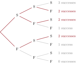
In the tree of $n$ independent trials, the binomial coefficient $\binom{n}{k}$ (read “ $n$ choose $k$ ”) is the number of paths containing exactly $k$ successes.

Example 19.5

$\binom{3}{2} = 3$ : the paths SSF, SFS, FSS. Likewise $\binom{3}{0} = 1$ (the path FFF), $\binom{3}{1} = 3$ and $\binom{3}{3} = 1$ . By convention and by the tree, $\binom n0 = \binom nn = 1$ for every $n$ .

The tree of n = 3 trials: 32 = 3 paths (red) carry exactly two successes, each with probability p2(1-p). — The tree of $n = 3$ trials: $\binom{3}{2} = 3$ paths (red) carry exactly two successes, each with probability $p^2(1-p)$ .

Proposition 19.6 (Pascal’s rule)

For $1 \leq k \leq n - 1$ :

\binom{n}{k} = \binom{n-1}{k-1} + \binom{n-1}{k}.

Proof. Sort the paths of the $n$ -trial tree with $k$ successes according to their last trial. Those ending in a success are obtained from a path of the first $n-1$ trials with $k - 1$ successes: there are $\binom{n-1}{k-1}$ of them. Those ending in a failure extend a path with $k$ successes among the first $n-1$ trials: $\binom{n-1}{k}$ of them. Every path is of exactly one of the two kinds. ∎

Pascal’s rule generates the coefficients row by row — each entry is the sum of the two above it:

\begin{array}{ccccccccccc} &&&&&1&&&&&\\ &&&&1&&1&&&&\\ &&&1&&2&&1&&&\\ &&1&&3&&3&&1&&\\ &1&&4&&6&&4&&1&\\ 1&&5&&10&&10&&5&&1 \end{array}

Remark 19.7

A closed formula, $\binom nk = \frac{n!}{k!(n-k)!}$ , together with a systematic theory of counting, is established in Chapter 27. At this level, Pascal’s triangle computes every coefficient we need.

19.3 The binomial distribution

Theorem 19.8 (Binomial distribution)

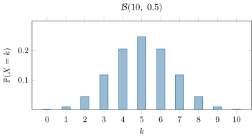
Let $X$ count the successes in $n$ independent Bernoulli trials of parameter $p$ . Then $X$ follows the binomial distribution $\mathcal B(n, p)$ :

\P(X = k) = \binom{n}{k}\, p^k (1-p)^{n-k}, \qquad k = 0, 1, \dots, n .

Proof. The event $X = k$ is the collection of all paths with exactly $k$ successes. Each such path has probability $p^k(1-p)^{n-k}$ : the product along the path contains $k$ factors $p$ and $n - k$ factors $1-p$ , in some order (Definition 19.2). There are $\binom nk$ such paths (Definition 19.4), and their probabilities add up. ∎

Example 19.9

A quiz has $5$ independent questions, each with $4$ choices; a student answers at random, so each question is a success with $p = \frac14$ . The number $X$ of correct answers follows $\mathcal B\left(5, \frac14\right)$ , and, using row $5$ of Pascal’s triangle:

\P(X = 2) = \binom52 \left(\frac14\right)^2\left(\frac34\right)^3 = 10 \times \frac{1}{16} \times \frac{27}{64} = \frac{270}{1024} \approx 0.26 .

The probability of at least one correct answer uses the complement: $\P(X \geq 1) = 1 - \P(X = 0) = 1 - \left(\frac34\right)^5 \approx 0.76$ .

Proposition 19.10 (Expectation and variance)

If $X \sim \mathcal B(n, p)$ :

\E(X) = np, \qquad \V(X) = np(1-p).

Justification. Write $X = X_1 + X_2 + \dots + X_n$ , where $X_i$ equals $1$ if the $i$ -th trial succeeds: each $X_i$ is a Bernoulli variable of expectation $p$ (Definition 19.1). Averages add — summing the $n$ contributions gives $\E(X) = np$ . That variances also add for independent variables is true but more delicate: the variance formula is admitted at this level and proved in Chapter 34. ∎

The distribution B(10, 0.5) (ten fair coin tosses): centered at (X) = np = 5, symmetric, with nearly all the probability between 2 and 8. — The distribution $\mathcal B(10, 0.5)$ (ten fair coin tosses): centered at $\E(X) = np = 5$ , symmetric, with nearly all the probability between $2$ and $8$ .

Method 19.11 (Recognizing a binomial situation)

Before writing $X \sim \mathcal B(n, p)$ , check three ingredients: a fixed number $n$ of trials, decided in advance; each trial has two outcomes with the same success probability $p$ ; the trials are independent (with replacement, or separate devices). Drawing without replacement from a small population is not binomial — the probability changes at each draw (Exercise 18.6).

19.4 Sampling: is the observation surprising?

The binomial distribution answers a very practical question: if the success probability really is $p$ , what counts of successes are plausible?

Example 19.12

A machine is supposed to produce $10\%$ defective items at most. In a batch of $10$ items, $4$ are defective. Bad luck or broken machine? If the machine is fine, the number of defectives follows $\mathcal B(10, 0.1)$ , and

\P(X \geq 4) = 1 - \P(X \leq 3) \approx 1 - 0.987 = 0.013 :

about one chance in $80$ . Observing an event this unlikely is a strong signal — one rejects the hypothesis that the machine still works at $10\%$ , while keeping in mind that the decision could be wrong with probability about $0.013$ .

Method 19.13 (Decision rule from a binomial model)

To judge an observed number $k$ of successes against a hypothesis $X \sim \mathcal B(n, p)$ : compute the probability, under the hypothesis, of a result at least as extreme as $k$ . If that probability is very small (a common convention: below $5\%$ ), reject the hypothesis; otherwise the observation is compatible with it. The threshold is a choice, not a theorem — statistics quantifies the risk, and the user accepts it.

19.5 Exercises

Exercise 19.1 ★

Extend Pascal’s triangle to row $7$ , and give the values of $\binom62$ , $\binom{7}{3}$ and $\binom74$ .

Solution

Solution of Exercise 19.1.

Rows $6$ and $7$ :

1,\ 6,\ 15,\ 20,\ 15,\ 6,\ 1 \qquad\text{and}\qquad 1,\ 7,\ 21,\ 35,\ 35,\ 21,\ 7,\ 1 .

Hence $\binom62 = 15$ , $\binom73 = 35$ , $\binom74 = 35$ (the symmetry $\binom73 = \binom74$ reflects swapping successes and failures).

Exercise 19.2 ★

A fair die is rolled $4$ times; $X$ counts the sixes. Justify that $X \sim \mathcal B\left(4, \frac16\right)$ and compute $\P(X = 0)$ , $\P(X = 1)$ and $\P(X \geq 2)$ .

Solution

Solution of Exercise 19.2.

Fixed number of trials ( $4$ rolls), two outcomes per roll (six or not, $p = \frac16$ ), independent rolls: $X \sim \mathcal B(4, \frac16)$ .

\P(X=0) = \left(\frac56\right)^4 = \frac{625}{1296} \approx 0.48, \qquad \P(X=1) = 4 \times \frac16\left(\frac56\right)^3 = \frac{500}{1296} \approx 0.39,

\P(X \geq 2) = 1 - \frac{625 + 500}{1296} = \frac{171}{1296} \approx 0.13 .

Exercise 19.3 ★

Which of the following is binomial? Justify.

Number of heads in $20$ tosses of a fair coin.
Number of aces in $5$ cards dealt from one deck.
Number of rainy days next week, if each day is rainy with probability $0.3$ independently.

Solution

Solution of Exercise 19.3.

1. Binomial $\mathcal B(20, \frac12)$ : fixed $n$ , same $p$ , independent tosses.

2. Not binomial: the cards are dealt without replacement, so the probability of an ace changes from card to card and the draws are not independent.

3. Binomial $\mathcal B(7, 0.3)$ by the stated independence assumption.

Exercise 19.4 ★

$X \sim \mathcal B(50, 0.2)$ . Give $\E(X)$ , $\V(X)$ and $\sigma(X)$ .

Solution

Solution of Exercise 19.4.

$\E(X) = 50 \times 0.2 = 10$ ; $\V(X) = 50 \times 0.2 \times 0.8 = 8$ ; $\sigma(X) = 2\sqrt2 \approx 2.83$ .

Exercise 19.5 ★★

An archer hits the target with probability $0.7$ at each shot, independently. In $6$ shots, compute the probability of exactly $4$ hits, and of at least $5$ hits.

Solution

Solution of Exercise 19.5.

$X \sim \mathcal B(6, 0.7)$ .

\P(X = 4) = \binom64 (0.7)^4 (0.3)^2 = 15 \times 0.2401 \times 0.09 \approx 0.324 .

\P(X \geq 5) = \binom65 (0.7)^5(0.3) + (0.7)^6 = 6 \times 0.16807 \times 0.3 + 0.117649 \approx 0.420 .

Exercise 19.6 ★★

A true/false test has $8$ questions; a student guesses each answer. What is the probability of passing (at least $6$ correct answers)?

Solution

Solution of Exercise 19.6.

$X \sim \mathcal B\left(8, \frac12\right)$ ; every path has probability $\frac{1}{256}$ , so

\P(X \geq 6) = \frac{\binom86 + \binom87 + \binom88}{256} = \frac{28 + 8 + 1}{256} = \frac{37}{256} \approx 0.14 .

Guessing passes about one time in seven.

Exercise 19.7 ★★

Each purchased cereal box contains figurine A or figurine B, with probability $\frac12$ each, independently. A collector buys $5$ boxes. Compute the probability that the collector gets at least one figurine of each kind. (Complement: all A or all B.)

Solution

Solution of Exercise 19.7.

The complement of “at least one of each” is “all five identical”: all A or all B, each with probability $\left(\frac12\right)^5 = \frac1{32}$ . Hence

\P(\text{one of each kind}) = 1 - \frac{2}{32} = \frac{15}{16} .

Exercise 19.8 ★★

A basketball player scores free throws with probability $p$ , independently. Let $X \sim \mathcal B(3, p)$ be the number of scores in three throws. Express $\P(X = 3)$ and $\P(X \geq 1)$ as functions of $p$ , and find for which $p$ the probability of scoring all three equals $\frac{27}{64}$ .

Solution

Solution of Exercise 19.8.

$\P(X = 3) = p^3$ and $\P(X \geq 1) = 1 - (1-p)^3$ . Solving $p^3 = \frac{27}{64} = \left(\frac34\right)^3$ gives $p = \frac34$ (the cube function is strictly increasing, Chapter 11, so the solution is unique).

Exercise 19.9 ★★

How many times must a fair coin be tossed for the probability of getting at least one head to exceed $0.99$ ? (Complement, then try successive values of $n$ .)

Solution

Solution of Exercise 19.9.

$\P(\text{at least one head}) = 1 - \left(\frac12\right)^n$ , so the condition is $\left(\frac12\right)^n < 0.01$ , i.e. $2^n > 100$ . Since $2^6 = 64$ and $2^7 = 128$ : from $n = 7$ tosses on.

Exercise 19.10 ★★

Using Pascal’s rule (Proposition 19.6) and $\binom n0 = \binom nn = 1$ , prove that the entries of each row of Pascal’s triangle sum to $2^n$ : interpret both sides as counting all the paths of the tree.

Solution

Solution of Exercise 19.10.

The sum of row $n$ counts all paths of the $n$ -trial tree, sorted by their number of successes. But the tree doubles its paths at each trial (each path splits into S and F), so it has $2^n$ paths in total. Hence $\sum_{k} \binom nk = 2^n$ . Alternatively, by induction: row $0$ sums to $1 = 2^0$ , and Pascal’s rule makes each entry of row $n$ contribute to exactly two entries of row $n+1$ , so the row sums double.

Exercise 19.11 ★★★

A politician claims $60\%$ approval. In a random sample of $10$ people, only $3$ approve.

Under the claim, what distribution does the number $X$ of approvals in the sample follow? Compute $\P(X \leq 3)$ .
Using the decision rule of Method 19.13 with a $5\%$ threshold, is the observation compatible with the claim?

Solution

Solution of Exercise 19.11.

1. Under the claim, $X \sim \mathcal B(10, 0.6)$ . Summing the first terms:

\begin{align*} \P(X \leq 3) &= (0.4)^{10} + 10(0.6)(0.4)^9 + 45(0.6)^2(0.4)^8 + 120(0.6)^3(0.4)^7\\ &\approx 0.0001 + 0.0016 + 0.0106 + 0.0425 = 0.0548 . \end{align*}

2. A result at least as extreme as the one observed ( $3$ or fewer approvals) has probability about $5.5\%$ — just above the $5\%$ threshold. Strictly applying the rule, the observation is (barely) compatible with the claim and one does not reject it. The example shows how sensitive borderline decisions are to the choice of threshold: with a $6\%$ convention the conclusion would flip.

19.6 Problem: The Galton board

Problem 19.1

Weekend problem — balls, pegs and Pascal’s triangle: how the bell shape is born, why playoff series favor the stronger team, and when to cry foul

Drop a thousand balls through a lattice of pegs, each bounce a fair left-or-right coin flip, and the slots below fill into a smooth, symmetric bell — every time. The machine is called a Galton board, and its mathematics is exactly this chapter’s binomial distribution (Theorem 19.8). This problem builds the triangle, runs the board, referees a best-of-seven series, and ends where the binomial earns its salary: deciding when an observation should make us doubt a claim.

Part I — The triangle.

Build Pascal’s triangle down to row $6$ (Proposition 19.6). State and explain the symmetry $\binom nk = \binom{n}{n-k}$ in one sentence (choosing $k$ objects is the same as …).
Verify on rows $4$ and $5$ that each row sums to $2^n$ , and prove it: what do all the $\binom nk$ together count?
Re-derive Pascal’s rule $\binom{n+1}{k} = \binom nk + \binom{n}{k-1}$ by the committee argument: fix one distinguished person and split the committees according to that person’s fate.
Compute $\binom73$ twice: from the triangle, and from the factorial formula.
Check the staircase identity $\binom22 + \binom32 + \binom42 + \binom52 = \binom63$ , and explain it by cascading Pascal’s rule from $\binom63$ downward.

Part II — The board. A ball falls through $n$ rows of pegs; at each peg it bounces left or right with probability $\frac12$ , independently. Number the slots $0$ to $n$ by the count of right bounces.

Explain, with the checklist of Method 19.11, why the slot number follows the binomial distribution $\mathcal B\!\left(n, \frac12\right)$ .
For a small board ( $n = 4$ ): give the five slot probabilities. Which slot is the most crowded?
Now $n = 10$ and $1\,024$ balls: what are the expected ball counts in the middle slot, in slot $7$ , and in each edge slot? Describe the pile’s shape.
For $X \sim \mathcal B\!\left(10, \frac12\right)$ : compute $\E(X)$ , $V(X)$ and $\sigma$ (Proposition 19.10); then compute the proportion of balls expected within $2\sigma$ of the center (slots $2$ to $8$ ) and compare with Chebyshev’s guarantee from Problem 17.1.
A tilted board bounces right with probability $0.6$ : give $\E$ , $V$ and $\sigma$ for $n = 10$ , and describe what happens to the pile.
In one or two sentences: what, in the board’s design, manufactures the bell shape — and why do so many real-world quantities (heights, measurement errors) pile up the same way? (The deep theorem behind both is the central limit theorem, the summit of the university volumes’ probability course.)

Part III — Best of seven. Two teams play a series: first to $4$ wins takes the title; games are independent.

Equal teams ( $p = \frac12$ ): compute the probability that the series ends in a sweep (exactly $4$ games).
Compute the probability that the series goes the full $7$ games (what must the score be after $6$ ?).
Complete the distribution of the series’ length ( $4$ , $5$ , $6$ or $7$ games) for equal teams, and compute the expected length. Which lengths are most likely?
Now one team wins each game with $p = 0.6$ . Compute its probability of taking the series (win in $4$ , $5$ , $6$ or $7$ : in each case the team wins the last game and $3$ of the previous ones). What did the series do to the per-game edge?
Compare with a single final ( $60\,\%$ ) and a best-of-3 (compute it). State the general effect of series length on skill against luck — and why leagues prefer long finals.

Part IV — When to cry foul.

A coin is flipped $100$ times and shows $62$ heads. For a fair coin, give $\E$ , $\sigma$ , and the z-score (Problem 17.1) of the observation. Verdict under the $2\sigma$ convention?
A supplier claims $2\,\%$ defective parts. In a batch of $50$ you find $3$ defective. Compute $\P(X \geq 3)$ under the claim ( $X \sim \mathcal B(50, 0.02)$ ; go through $\P(X = 0), \P(X = 1), \P(X = 2)$ ). Alarming at the $5\,\%$ threshold (Method 19.13, Exercise 19.11)?
Lottery persistence: each ticket wins (something) with probability $\frac{1}{1000}$ . Compute the probability of at least one win with $1\,000$ tickets. The answer ( $\approx 63\,\%$ , not $100\,\%$ !) hides a famous constant: compute $0.999^{1000}$ and keep the number $0.368$ in mind for grade 12.
Finale — the binomial’s portrait: the recognition checklist (fixed $n$ , independence, constant $p$ ); Pascal’s triangle as its table; the bell as its shape; $np$ and $np(1-p)$ as its compass; and its two heirs awaiting in grade 12 — the smooth bell curve and the law of large numbers. One sentence each.

Solution

Solution of Problem 19.1.

1. Rows: $1$ ; $1\,1$ ; $1\,2\,1$ ; $1\,3\,3\,1$ ; $1\,4\,6\,4\,1$ ; $1\,5\,10\,10\,5\,1$ ; $1\,6\,15\,20\,15\,6\,1$ . Symmetry: choosing which $k$ objects to take is the same act as choosing which $n - k$ to leave behind.

2. $1 + 4 + 6 + 4 + 1 = 16 = 2^4$ ; $1 + 5 + 10 + 10 + 5 + 1 = 32 = 2^5$ . Proof: the $\binom nk$ count the subsets of each size of an $n$ -element set, and the subsets altogether number $2^n$ (each element in or out, independently).

3. Committees of $k$ chosen among $n + 1$ people, one of whom is Zoe: those without Zoe are $\binom nk$ (choose all $k$ among the others); those with Zoe are $\binom{n}{k-1}$ (choose her $k - 1$ colleagues). Total: $\binom nk + \binom{n}{k-1}$ .

4. Triangle row $7$ : $1\,7\,21\,35\,\dots$ : $35$ . Formula: $\frac{7 \times 6 \times 5}{3 \times 2 \times 1} = 35$ .

5. $1 + 3 + 6 + 10 = 20 = \binom63$ . Cascade: $\binom63 = \binom52 + \binom53 = \binom52 + \binom42 + \binom43 = \binom52 + \binom42 + \binom32 + \binom33$ — each application of Pascal’s rule peels off one term of the staircase.

6. Fixed number $n$ of bounces; each bounce an independent Bernoulli trial with the same $p = \frac12$ ; the slot number counts the successes (right bounces): all three boxes of Method 19.11 ticked: $\mathcal B\!\left(n, \frac12\right)$ .

7. Probabilities $\frac{1}{16}, \frac{4}{16}, \frac{6}{16}, \frac{4}{16}, \frac{1}{16}$ for slots $0, \dots, 4$ : the center slot $2$ is the most crowded.

8. Expected counts $= 1024 \times \binom{10}{k}/1024 = \binom{10}{k}$ : middle slot $\binom{10}{5} = 252$ balls; slot $7$ : $\binom{10}{7} = 120$ ; each edge slot: $1$ ball. A tall center falling away symmetrically to whisper-thin edges: the bell.

9. $\E = np = 5$ ; $V = np(1 - p) = 2.5$ ; $\sigma \approx 1.58$ . Within $2\sigma$ : slots $2$ to $8$ carry

\frac{45 + 120 + 210 + 252 + 210 + 120 + 45}{1024} = \frac{1002}{1024} \approx 98\,\%

of the balls — far better than Chebyshev’s all-purpose $75\,\%$ (Problem 17.1): bell shapes concentrate hard.

10. $\E = 6$ , $V = 10 \times 0.6 \times 0.4 = 2.4$ , $\sigma \approx 1.55$ : the pile keeps its bell shape but slides its summit to slot $6$ — a tilted board is a loaded coin made visible.

11. The slot number is a sum of many small, independent, same-sized chance pushes — and such sums always organize themselves into the bell: most pushes cancel, extremes require unanimity. Heights, measurement errors and countless natural quantities are likewise sums of many small independent effects, which is why the same silhouette appears everywhere; the theorem certifying it is the central limit theorem.

12. A sweep: one team wins all $4$ : $2 \times \left(\frac12\right)^4 = \frac18$ .

13. Seven games require $3$ – $3$ after six: $\binom63 \left(\frac12\right)^6 = \frac{20}{64} = \frac{5}{16}$ .

14. Ends in $5$ : the winner takes game 5 and $3$ of the first $4$ : $2 \times \binom43 \left(\frac12\right)^5 = \frac14$ . Ends in $6$ : $2 \times \binom53 \left(\frac12\right)^6 = \frac{5}{16}$ . Distribution over $4, 5, 6, 7$ : $\frac18, \frac14, \frac{5}{16}, \frac{5}{16}$ (sum $1$ ). Expected length: $4 \cdot \frac18 + 5 \cdot \frac14 + 6 \cdot \frac{5}{16} + 7 \cdot \frac{5}{16} = 5.8125$ games. Six- and seven-game series are the most likely — drama is built into the format.

15. Win in $4$ : $0.6^4 = 0.1296$ ; in $5$ : $\binom43\,0.6^3 \times 0.4 \times 0.6 = 0.2074$ ; in $6$ : $\binom53\,0.6^3 \times 0.4^2 \times 0.6 = 0.2074$ ; in $7$ : $\binom63\,0.6^3 \times 0.4^3 \times 0.6 = 0.1659$ . Total: about $0.710$ : a $60\,\%$ -per-game team wins $71\,\%$ of series — the series amplifies the edge.

16. Single final: $60\,\%$ . Best-of-3: $p^2 + 2p^2 q = 0.36 + 0.288 = 0.648$ . The ladder $60\,\% \to 65\,\% \to 71\,\%$ continues with length: more games average out luck (the law of large numbers in miniature), so long finals crown skill — which is precisely what leagues sell.

17. Fair coin: $\E = 50$ , $\sigma = \sqrt{25} = 5$ ; $z = \frac{62 - 50}{5} = 2.4$ : beyond the $2\sigma$ convention — the coin deserves an investigation.

18. $\P(X = 0) = 0.98^{50} \approx 0.364$ ; $\P(X = 1) = 50 \times 0.02 \times 0.98^{49} \approx 0.372$ ; $\P(X = 2) = \binom{50}{2} 0.02^2 \times 0.98^{48} \approx 0.186$ . So $\P(X \geq 3) \approx 1 - 0.922 = 0.078$ : about $7.8\,\%$ — above the $5\,\%$ threshold, so not (yet) enough to reject the claim; a second bad batch would change the story.

19. $\P(\text{at least one win}) = 1 - 0.999^{1000} \approx 1 - 0.368 = 0.632$ : a thousand tickets at one in a thousand give not certainty but $63\,\%$ . The recurring $0.368$ is $\frac1e$ in disguise — the constant $e$ makes its official entrance in grade 12.

20. Recognition: fixed $n$ , independence, constant $p$ — then and only then, binomial. Table: Pascal’s triangle, row $n$ . Shape: the bell, symmetric for $p = \frac12$ , shifted otherwise. Compass: center $np$ , spread $\sqrt{np(1-p)}$ — the z-scores of decisions. Heirs: the smooth bell curve that the piles approach, and the law of large numbers that explains why big boards never lie.