High School Mathematics · Grades 10–12

35Continuous Random Variables

Waiting times, physical measurements, proportions: many random quantities take a continuum of values, and no single value has positive probability. Probabilities are then computed by integrating a density. This chapter studies the uniform, exponential and normal distributions, and uses the normal law to quantify the fluctuations of polls and samples.

35.1 Probability densities

Definition 35.1 (Density, continuous random variable)

A probability density on an interval $I$ is a continuous, nonnegative function $f$ on $I$ with $\int_I f(t)\,\dd t = 1$ (the integral over an unbounded $I$ being understood as a limit of integrals over growing bounded intervals). A random variable $X$ has density $f$ if for all $a \leq b$ in $I$ :

\P(a \leq X \leq b) = \int_a^b f(t)\,\dd t .

Probabilities are areas under the density curve. In particular $\P(X = a) = \int_a^a f = 0$ for every single value $a$ : only intervals carry probability, and $\P(a \leq X \leq b) = \P(a < X < b)$ .

Definition 35.2 (Expectation and variance)

For $X$ with density $f$ on $I$ :

\E(X) = \int_I t\,f(t)\,\dd t, \qquad \V(X) = \int_I \bigl(t - \E(X)\bigr)^2 f(t)\,\dd t = \E(X^2) - \E(X)^2 .

The rules of Chapters 14–15 (linearity of expectation, additivity of variance for independent variables, Bienaymé–Chebyshev) remain valid; their proofs, with integrals in place of sums, are admitted at this level.

35.2 Uniform distribution

Definition 35.3 (Uniform distribution)

$X$ follows the uniform distribution $\mathcal U\intcc ab$ if its density is constant, $f(t) = \frac{1}{b-a}$ on $\intcc{a}{b}$ . Then for $\intcc{c}{d} \subseteq \intcc ab$ , $\P(c \leq X \leq d) = \frac{d - c}{b - a}$ : probability proportional to length.

Proposition 35.4

If $X \sim \mathcal U\intcc ab$ , then $\E(X) = \dfrac{a+b}{2}$ and $\V(X) = \dfrac{(b-a)^2}{12}$ .

Proof. $\E(X) = \int_a^b \frac{t}{b-a}\dd t = \frac{b^2 - a^2}{2(b-a)} = \frac{a+b}{2}$ . For the variance, $\E(X^2) = \frac{b^3 - a^3}{3(b-a)} = \frac{a^2 + ab + b^2}{3}$ , and

\V(X) = \frac{a^2 + ab + b^2}{3} - \frac{(a+b)^2}{4} = \frac{4a^2 + 4ab + 4b^2 - 3a^2 - 6ab - 3b^2}{12} = \frac{(b - a)^2}{12}. \qedhere

∎

35.3 Exponential distribution

Definition 35.5 (Exponential distribution)

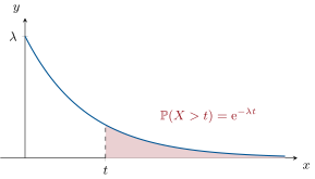
For $\lambda > 0$ , $X$ follows the exponential distribution $\mathcal E(\lambda)$ if its density on $\intco{0}{+\infty}$ is

f(t) = \lambda\,\eu^{-\lambda t}.

Then $\P(X \leq x) = 1 - \eu^{-\lambda x}$ and $\P(X > x) = \eu^{-\lambda x}$ for $x \geq 0$ .

Proposition 35.6

If $X \sim \mathcal E(\lambda)$ : $\E(X) = \dfrac{1}{\lambda}$ and $\V(X) = \dfrac{1}{\lambda^2}$ .

Proof. Integrating by parts on $\intcc{0}{A}$ :

\int_0^A t\,\lambda\eu^{-\lambda t}\dd t = \bigl[-t\,\eu^{-\lambda t}\bigr]_0^A + \int_0^A \eu^{-\lambda t}\dd t = -A\eu^{-\lambda A} + \frac{1 - \eu^{-\lambda A}}{\lambda} \xrightarrow[A\to+\infty]{} \frac1\lambda,

using $A\eu^{-\lambda A} \to 0$ (Theorem 23.4). A second integration by parts gives $\E(X^2) = \frac{2}{\lambda^2}$ , whence $\V(X) = \frac{2}{\lambda^2} - \frac{1}{\lambda^2}$ . ∎

Theorem 35.7 (Memorylessness)

If $X \sim \mathcal E(\lambda)$ , then for all $s, t \geq 0$ :

\pcond{X > s}{X > s + t} = \P(X > t) .

The exponential distribution is the law of lifetimes without aging (radioactive nuclei, not light bulbs).

Proof.

\pcond{X > s}{X > s+t} = \frac{\P(X > s + t)}{\P(X > s)} = \frac{\eu^{-\lambda(s+t)}}{\eu^{-\lambda s}} = \eu^{-\lambda t} = \P(X > t). \qedhere

∎

The exponential density - x (here = 1): the tail area beyond t (red) is - t, and memorylessness says every tail looks like the whole distribution rescaled. — The exponential density $\lambda\eu^{-\lambda x}$ (here $\lambda = 1$ ): the tail area beyond $t$ (red) is $\eu^{-\lambda t}$ , and memorylessness says every tail looks like the whole distribution rescaled.

35.4 Normal distribution

Definition 35.8 (Normal distribution)

$X$ follows the standard normal distribution $\mathcal N(0, 1)$ if its density on $\R$ is

\varphi(t) = \frac{1}{\sqrt{2\pi}}\,\eu^{-t^2/2}

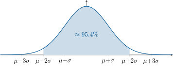
(the bell curve). More generally, $X \sim \mathcal N(\mu, \sigma^2)$ if $\dfrac{X - \mu}{\sigma} \sim \mathcal N(0,1)$ ; then $\E(X) = \mu$ and $\V(X) = \sigma^2$ .

The normal density: about 68.3\% of the mass lies within of the mean, 95.4\% within 2, 99.7\% within 3. — The normal density: about $68.3\%$ of the mass lies within $\sigma$ of the mean, $95.4\%$ within $2\sigma$ , $99.7\%$ within $3\sigma$ .

Remark 35.9

The factor $\frac{1}{\sqrt{2\pi}}$ makes the total area $1$ — a famous computation (the Gaussian integral) done at university. There is no elementary formula for $\int \varphi$ : normal probabilities are read from tables or calculators.

Theorem 35.10 (De Moivre–Laplace, admitted)

Let $X_n \sim \mathcal B(n, p)$ and $Z_n = \dfrac{X_n - np}{\sqrt{np(1-p)}}$ (the standardized binomial). Then for all $a \leq b$ ,

\P(a \leq Z_n \leq b) \xrightarrow[n\to+\infty]{} \int_a^b \varphi(t)\,\dd t .

This result is admitted at this level. It explains the universal appearance of the bell curve: a binomial with large $n$ is approximately normal — and (central limit theorem, university) so is any sum of many small independent effects.

Method 35.11 (Fluctuation interval at $95\%$ )

Since a normal variable falls within $1.96$ standard deviations of its mean with probability $0.95$ , for $n$ large a frequency $F_n = \frac{X_n}{n}$ of a $\mathcal B(n,p)$ sample satisfies

\P\left(p - 1.96\sqrt{\tfrac{p(1-p)}{n}} \leq F_n \leq p + 1.96\sqrt{\tfrac{p(1-p)}{n}}\right) \approx 0.95 .

Fluctuation interval (testing): if a claimed $p$ puts the observed frequency outside this interval, reject the claim at the $5\%$ level.
Confidence interval (estimating): the simplified interval $\left[F_n - \frac{1}{\sqrt n},\ F_n + \frac{1}{\sqrt n}\right]$ contains $p$ with probability at least $0.95$ (using $1.96\sqrt{p(1-p)} \leq 1$ , see Exercise 34.8).

Example 35.12

A poll of $n = 1000$ voters gives a candidate $52\%$ . The confidence interval $52\% \pm \frac{1}{\sqrt{1000}} \approx 52\% \pm 3.2\%$ still contains $50\%$ : the poll alone does not establish that the candidate is ahead.

35.5 Exercises

Exercise 35.1 ★

A bus passes every $15$ minutes; a traveler arrives at a uniformly random time. Let $X \sim \mathcal U\intcc{0}{15}$ be the waiting time. Compute $\P(X \leq 5)$ , $\P(4 \leq X \leq 10)$ , $\E(X)$ and $\sigma(X)$ .

Solution

Solution of Exercise 35.1.

$\P(X \leq 5) = \frac{5}{15} = \frac13$ ; $\P(4 \leq X \leq 10) = \frac{6}{15} = \frac25$ ; $\E(X) = \frac{15}{2} = 7.5$ min; $\sigma(X) = \frac{15}{\sqrt{12}} = \frac{5\sqrt3}{2} \approx 4.3$ min.

Exercise 35.2 ★

Check that $f(t) = \frac{3}{8}t^2$ is a density on $\intcc{0}{2}$ , and compute $\E(X)$ and $\P(X \geq 1)$ for a variable $X$ with this density.

Solution

Solution of Exercise 35.2.

$f \geq 0$ and $\int_0^2 \frac38 t^2\,\dd t = \frac38\left[\frac{t^3}{3}\right]_0^2 = \frac38 \times \frac83 = 1$ : a density.

\E(X) = \int_0^2 \frac38 t^3\,\dd t = \frac38 \times \frac{16}{4} = \frac32, \qquad \P(X \geq 1) = \int_1^2 \frac38 t^2\,\dd t = \frac{8 - 1}{8} = \frac78 .

Exercise 35.3 ★

The lifetime (in years) of an electronic component follows $\mathcal E(0.2)$ .

Compute the expected lifetime and $\P(X > 5)$ .
The component has already worked $3$ years. What is the probability it works at least $5$ more?

Solution

Solution of Exercise 35.3.

1. $\E(X) = \frac{1}{0.2} = 5$ years; $\P(X > 5) = \eu^{-0.2\times5} = \eu^{-1} \approx 0.37$ .

2. By memorylessness (Theorem 35.7), $\pcond{X > 3}{X > 8} = \P(X > 5) = \eu^{-1} \approx 0.37$ : the three years of service change nothing.

Exercise 35.4 ★★

The half-life of a radioactive atom whose lifetime follows $\mathcal E(\lambda)$ is the median $m$ : $\P(X > m) = \frac12$ . Express $m$ as a function of $\lambda$ and compare with the expectation. Which is larger, and why does that make sense for a skewed distribution?

Solution

Solution of Exercise 35.4.

$\P(X > m) = \eu^{-\lambda m} = \frac12$ gives $m = \frac{\ln 2}{\lambda} \approx \frac{0.69}{\lambda}$ , smaller than $\E(X) = \frac1\lambda$ . The exponential density has a long right tail: a few atypically long lifetimes pull the mean above the median, the value that half the population exceeds. (This is the half-life of Example 23.9: half the atoms survive it, even though the average lifetime is longer.)

Exercise 35.5 ★★

Heights in a population follow $\mathcal N(175,\ 7^2)$ (in cm). Using the $68$ – $95$ – $99.7$ rule, estimate the proportion of the population with height between $168$ and $182$ cm, above $189$ cm, and below $154$ cm.

Solution

Solution of Exercise 35.5.

$168 = \mu - \sigma$ and $182 = \mu + \sigma$ : about $68\%$ . $189 = \mu + 2\sigma$ : above it lies half of the remaining $100 - 95.4 = 4.6\%$ , so about $2.3\%$ . $154 = \mu - 3\sigma$ : about $\frac{100 - 99.7}{2} = 0.15\%$ .

Exercise 35.6 ★★

A machine fills bags labeled $500$ g; the mass filled follows $\mathcal N(\mu,\ 4^2)$ . Regulations demand that at most $2.5\%$ of bags weigh less than $500$ g. Using the $95\%$ rule, what minimal setting of $\mu$ complies?

Solution

Solution of Exercise 35.6.

$\P(X < 500) \leq 2.5\%$ means $500$ must sit at least two standard deviations below the mean (the normal leaves $2.3\% \approx 2.5\%$ below $\mu - 2\sigma$ ; with the conventional $1.96$ , the reasoning is identical):

\mu - 2\sigma \geq 500 \iff \mu \geq 500 + 8 = 508 \text{ g}.

The machine must be set to $508$ g on average — the price of the guarantee is $8$ g of “free” product per bag.

Exercise 35.7 ★★

A die claimed to be fair is rolled $1200$ times and shows a six $260$ times (as in Exercise 34.7).

Compute the $95\%$ fluctuation interval for the frequency of sixes of a fair die over $1200$ rolls.
Is the observed frequency inside? Compare the strength of this conclusion with the Bienaymé–Chebyshev analysis.

Solution

Solution of Exercise 35.7.

1. With $p = \frac16$ , $n = 1200$ : $\sqrt{\frac{p(1-p)}{n}} = \sqrt{\frac{5/36}{1200}} \approx 0.0108$ , so the $95\%$ fluctuation interval is

\frac16 \pm 1.96 \times 0.0108 \approx \intcc{0.146}{0.188}.

2. The observed frequency $\frac{260}{1200} \approx 0.217$ lies far outside: the fairness hypothesis is rejected at the $5\%$ level. The deviation is about $4.6$ standard deviations — for a normal approximation, a probability of order $10^{-6}$ , far more conclusive than the $\leq 4.6\%$ bound from Bienaymé–Chebyshev (Exercise 34.7).

Exercise 35.8 ★★★

Before an election, a poll of $n$ people will estimate the score $p$ of a candidate by the observed frequency $F_n$ .

With the confidence interval of Method 35.11, what sample size guarantees a margin of $\pm 2$ points?
The candidates are separated by $1$ point in reality. Explain why no realistic poll can reliably call the winner, however well conducted.

Solution

Solution of Exercise 35.8.

1. Margin $\frac{1}{\sqrt n} \leq 0.02$ requires $n \geq 2500$ people.

2. To distinguish scores $1$ point apart, the margin must be well under $0.5$ point, requiring $n \geq \left(\frac{1}{0.005}\right)^2 = 40\,000$ by the simplified formula — already impractical for most polls. Worse, the statistical margin only accounts for sampling error; systematic biases (unrepresentative samples, non-response, last-minute swings) do not shrink as $n$ grows and typically exceed one point. A $1$ -point race is genuinely too close to call.

Exercise 35.9 ★★★

Let $X$ have density $f$ on $\intcc ab$ and let $Y = \alpha X + \beta$ with $\alpha > 0$ .

Show that $\P(c \leq Y \leq d) = \P\left(\frac{c - \beta}{\alpha} \leq X \leq \frac{d-\beta}{\alpha}\right)$ , and deduce that $Y$ has density $g(y) = \frac{1}{\alpha} f\left(\frac{y - \beta}{\alpha}\right)$ .
Deduce that if $Z \sim \mathcal N(0,1)$ , then $\mu + \sigma Z$ has density $\frac{1}{\sigma\sqrt{2\pi}}\, \eu^{-(y - \mu)^2/(2\sigma^2)}$ — the general normal density.

Solution

Solution of Exercise 35.9.

1. Since $\alpha > 0$ , $c \leq \alpha X + \beta \leq d \iff \frac{c - \beta}{\alpha} \leq X \leq \frac{d - \beta}{\alpha}$ , so

\P(c \leq Y \leq d) = \int_{(c-\beta)/\alpha}^{(d-\beta)/\alpha} f(t)\,\dd t .

The substitution $y = \alpha t + \beta$ (i.e. reading the area in the $y$ variable, $t = \frac{y - \beta}{\alpha}$ , $\dd t = \frac{\dd y}{\alpha}$ ) turns this into $\int_c^d \frac{1}{\alpha} f\left(\frac{y-\beta}{\alpha}\right)\dd y$ : the function $g(y) = \frac1\alpha f\left(\frac{y-\beta}{\alpha}\right)$ is a density of $Y$ .

2. With $f = \varphi$ , $\alpha = \sigma$ , $\beta = \mu$ :

g(y) = \frac{1}{\sigma}\,\varphi\!\left(\frac{y - \mu}{\sigma}\right) = \frac{1}{\sigma\sqrt{2\pi}}\, \exp\left(-\frac{(y-\mu)^2}{2\sigma^2}\right),

which is therefore the density of $\mathcal N(\mu, \sigma^2) = \mu + \sigma\,\mathcal N(0,1)$ .

35.6 Problem: Waiting for the bus, measuring the crowd

Problem 35.1

Weekend problem — three densities run the world: total ignorance, memoryless waiting, and the bell of many small causes; plus the paradox that makes your bus always late

Why does your bus always seem to take longer than the timetable promises? Why is the class an average student sits in bigger than the average class? Why do your friends have more friends than you? One sly piece of mathematics — length-biased sampling — answers all three, and it lives in this chapter, between the uniform, exponential and normal distributions (Definition 35.3, Definition 35.5, Definition 35.8). This final problem of the volume puts the three densities to work and ends where the whole series points: the bell curve.

Part I — Three characters.

A bus arrives at a uniformly random time in the next $30$ minutes. Compute $\P(\text{wait} \leq 10)$ , the expected wait, and $\sigma$ (Proposition 35.4).
Check that $f(x) = 2x$ on $\intcc{0}{1}$ is a density, and compute $\E(X)$ and $\P\left(X > \frac12\right)$ .
Phone calls reach a helpline as a memoryless stream: the wait for the next call is exponential with mean $10$ minutes. Compute $\P(T > 15)$ and the median wait — why is the median less than the mean?
You have already waited $20$ minutes. What is $\P(T > 35 \mid T > 20)$ (Theorem 35.7)? Interpret in one sentence.
Match each wait to its right model — uniform, exponential, or neither: (a) the click of a Geiger counter; (b) a metro running every $8$ minutes, your arrival unsynchronized; (c) the next call at the helpline; (d) the failure of a light bulb that wears out. Justify (d) with the memorylessness theorem.

Part II — The bell at work. (Use the normal landmarks: $68\,\%$ within $\sigma$ , $95\,\%$ within $2\sigma$ , $99.7\,\%$ within $3\sigma$ .)

Adult heights follow roughly $\mathcal N(172,\ 8)$ (cm). What fractions lie in $\intcc{164}{180}$ , $\intcc{156}{188}$ , $\intcc{148}{196}$ ?
Estimate the proportion taller than $190$ cm (z-score first; table or calculator).
IQ scores are calibrated to $\mathcal N(100, 15)$ . What fraction scores above $130$ — and roughly one person in how many?
A machine cuts bolts with lengths $\mathcal N(50,\ 0.1)$ mm and the specification is $\intcc{49.8}{50.2}$ . What share is rejected? Industry celebrates “six sigma” processes, whose specifications sit at $\pm 6\sigma$ : what does that buy, and why do factories chase it?
De Moivre–Laplace (Theorem 35.10): for $100$ fair coin flips, approximate $\P(45 \leq \text{heads} \leq 55)$ (continuity: $\pm 0.5$ ; $\sigma = 5$ ). Which wooden machine of Problem 19.1 does this theorem smooth into a curve?
From Exercise 35.8: a $\pm 2$ -point margin needs about $n = 2\,400$ . Compute the sample needed for $\pm 0.5$ points — and conclude, in one sentence, why a race separated by one point cannot be honestly called by any poll.

Part III — The bus paradox.

Buses arrive as a memoryless stream with mean gap $10$ minutes. You reach the stop at an arbitrary moment. Intuition says the expected wait is $5$ minutes (half a gap). What does the memorylessness theorem say instead?
Diagnose the intuition with a toy timetable: gaps alternate $5$ and $15$ minutes (mean gap $10$ ). Compute the probability that a uniformly random arrival lands in a long gap, then the true expected wait — and name the culprit: arrivals sample gaps with probability proportional to their length.
In the memoryless stream, the gap you land in has expected length $20$ minutes — twice the typical gap (the time back to the previous bus and forward to the next are both exponential with mean $10$ ). Reconcile this with question 12 and state the inspection paradox in one sentence.
Same sting on land: a university runs nine classes of $10$ students and one of $110$ . Compute the average class size, then the class size experienced by the average student. Which number will the brochure quote, and which is the students’ lived truth?
The friendship paradox — “your friends have, on average, more friends than you” — is the same mathematics. Say in one sentence what plays the role of the long gap.

Part IV — Closing the volume.

Simulation, the practitioners’ bridge: if $U$ is uniform on $\intoo{0}{1}$ , show that $T = -10\ln U$ is exponential with mean $10$ (compute $\P(T > t)$ ). Every random-waiting simulation in industry runs on this one-line trick.
An old game programmers’ recipe builds a bell: add twelve independent uniforms on $\intcc{0}{1}$ and subtract $6$ . Give the mean and variance of the sum, and explain — Galton board in hand — why the result is nearly normal.
Markets crash harder than the bell allows: the 1987 crash was described as a “ $25\sigma$ event”, which under normality has probability around $10^{-137}$ . What is the correct conclusion — about the world, or about the model? (One sentence, the statistician’s catechism.)
Finale, and farewell to the volume: the three characters in one line each — uniform (ignorance within bounds), exponential (hazard without memory), normal (the sum of many small causes); the inspection paradox as the chapter’s sting; and the arc of the whole series — from counting cartons in grade 6 to the bell curve that measures every crowd — with the university volumes waiting where the limits, the integrals and the central limit theorem take over.

Solution

Solution of Problem 35.1.

1. $\P(\text{wait} \leq 10) = \frac{10}{30} = \frac13$ ; $\E = 15$ min; $\sigma = \frac{30}{\sqrt{12}} \approx 8.7$ min.

2. $\int_0^1 2x\,\dd x = 1$ : a density. $\E(X) = \int_0^1 2x^2\,\dd x = \frac23$ ; $\P\left(X > \frac12\right) = \int_{1/2}^1 2x\,\dd x = 1 - \frac14 = \frac34$ .

3. $\P(T > 15) = \eu^{-15/10} \approx 0.22$ . Median: $\eu^{-m/10} = \frac12$ : $m = 10\ln 2 \approx 6.9$ min — less than the mean $10$ because the exponential’s long right tail (rare huge waits) drags the mean upward while leaving the median at the “typical” wait.

4. By memorylessness, $\P(T > 35 \mid T > 20) = \P(T > 15) \approx 0.22$ : the twenty minutes already served buy nothing — the stream does not age.

5. (a) exponential (radioactive decay is the model memorylessness was invented for); (b) uniform on $\intcc{0}{8}$ (a schedule with a random offset); (c) exponential; (d) neither: a worn bulb is more likely to fail in the next hour than a new one, so $\P(T > s + t \mid T > s) < \P(T > t)$ : aging contradicts the memorylessness theorem.

6. $68\,\%$ , $95\,\%$ , $99.7\,\%$ : the three landmark intervals.

7. $z = \frac{190 - 172}{8} = 2.25$ : upper tail $\approx 1.2\,\%$ .

8. $z = 2$ : about $2.3\,\%$ — roughly one person in $44$ .

9. The spec sits at $\pm 2\sigma$ : about $95.4\,\%$ pass, $4.6\,\%$ rejected — ruinous at scale. At $\pm 6\sigma$ the failure rate drops to about two parts per billion: six-sigma buys the right to mass-produce without mass-inspecting.

10. $\sigma = 5$ ; with continuity correction, $\P \approx \P\left(\abs Z \leq \frac{5.5}{5}\right) = \P(\abs Z \leq 1.1) \approx 0.73$ . The theorem smooths the Galton board of Problem 19.1: the staircase of slots becomes the continuous bell.

11. $n \approx \frac{1.96^2 \times 0.25}{0.005^2} \approx 38\,400$ people — and at that size the non-sampling errors (frame, refusals, lies) dwarf the margin: a one-point race is beyond honest polling, which is why serious institutes then say “too close to call”.

12. Memorylessness: from the moment you arrive, the remaining wait is exponential with mean $10$ — the full $10$ minutes, not $5$ . The timetable’s “mean gap $10$ ” misleads: your wait has the same distribution as a whole gap.

13. Random arrivals land proportionally to gap length: $\P(\text{long gap}) = \frac{15}{20} = \frac34$ . Expected wait: $\frac34 \times \frac{15}{2} + \frac14 \times \frac52 = 5.625 + 0.625 = 6.25$ min — more than the naive $5$ , though the mean gap is $10$ . Culprit: length-biased sampling — long gaps catch more passengers.

14. Backward and forward waits are each exponential with mean $10$ (memorylessness runs in both directions from your arrival): the gap containing you averages $20$ minutes — twice the typical gap. Inspection paradox in one sentence: the interval you happen to inspect is not a typical interval, because you were more likely to fall into a big one.

15. Average class: $\frac{9 \times 10 + 110}{10} = 20$ students. Student-experienced average: $\frac{90 \times 10 + 110 \times 110}{200} = \frac{13\,000} {200} = 65$ students. The brochure prints $20$ ; three in five students sit in the class of $110$ and live the $65$ .

16. Popular people appear on many friend-lists, so sampling “a friend” is length-biased towards the sociable — your friends are drawn from the long gaps of the social timetable.

17. For $t \geq 0$ : $\P(T > t) = \P(-10\ln U > t) = \P\left(U < \eu^{-t/10}\right) = \eu^{-t/10}$ : exactly the exponential’s survival function — one logarithm converts the computer’s uniform noise into any waiting time.

18. Each uniform has mean $\frac12$ and variance $\frac{1}{12}$ : the sum of twelve has mean $6$ and variance $1$ — so the recipe outputs mean $0$ , variance $1$ . Twelve independent small pushes summed: the Galton mechanism, and by De Moivre–Laplace’s blessing the histogram is already bell-shaped to the eye.

19. About the model: markets are not sums of many independent small causes — panics correlate everything (the 2008 lesson of the previous problem) and produce fat tails no normal density owns. When the data whispers $10^{-137}$ , the statistician’s catechism answers: the model is rejected, not the day.

20. Uniform: all positions equal, the honest “I know only the bounds”. Exponential: the hazard that never ages — decays, arrivals, clicks. Normal: the democratic bell of many small independent causes — heights, errors, averages. Sting: what you sample is biased by how you bumped into it — buses, classes, friends. And the arc: the child who counted juice cartons in grade 6 has, ten volumes of problems later, measured the crowd with a curve; the epsilon, the integral and the central limit theorem are waiting in the university volumes to explain why the bell tolls for everything.