High School Mathematics · Grades 10–12

33Random Variables and the Binomial Distribution

A random variable attaches a number to each outcome of an experiment: a gain, a count, a duration. Its expectation is the long-run average of the values it produces, its variance measures their spread. The star of this chapter is the binomial distribution, which counts successes in repeated independent trials. Random variables and the binomial distribution were first met in Chapters 18 and 19; this chapter reviews and deepens them, with the combinatorial tools of Chapter 27 now available.

33.1 Discrete random variables

Definition 33.1 (Random variable, distribution)

A random variable on a finite sample space $\Omega$ is a function $X \colon \Omega \to \R$ . Its distribution (or law) is the data of its possible values $x_1, \dots, x_k$ and of the probabilities

p_i = \P(X = x_i), \qquad \sum_{i=1}^{k} p_i = 1 .

Definition 33.2 (Expectation, variance, standard deviation)

The expectation of $X$ is

\E(X) = \sum_{i=1}^{k} p_i\, x_i ,

its variance and standard deviation are

\V(X) = \E\bigl((X - \E(X))^2\bigr) = \sum_{i=1}^k p_i\bigl(x_i - \E(X)\bigr)^2, \qquad \sigma(X) = \sqrt{\V(X)} .

Proposition 33.3 (König–Huygens formula)

$\V(X) = \E(X^2) - \E(X)^2$ .

Proof. Write $m = \E(X)$ and expand:

\V(X) = \sum_i p_i (x_i^2 - 2m x_i + m^2) = \E(X^2) - 2m\sum_i p_i x_i + m^2\sum_i p_i = \E(X^2) - 2m^2 + m^2 . \qedhere

∎

Proposition 33.4 (Affine transformation)

For $a, b \in \R$ :

\E(aX + b) = a\,\E(X) + b, \qquad \V(aX + b) = a^2\,\V(X) .

Proof. The first is a rearrangement of the defining sum. For the second, $aX + b$ deviates from its mean by $a(X - \E(X))$ , and squaring multiplies by $a^2$ . ∎

Example 33.5 (Fair games)

A game costs $2$ euros; a die is rolled, and the player receives the value shown if it is at least $5$ , nothing otherwise. The gain $G$ takes values $-2$ (probability $\frac46$ ), $3$ ( $\frac16$ ), $4$ ( $\frac16$ ):

\E(G) = \frac{-8 + 3 + 4}{6} = -\frac{1}{6} < 0 .

On average, the player loses $17$ cents per game: the game is unfavorable (as most real games are).

33.2 Bernoulli trials and the binomial distribution

Definition 33.6 (Bernoulli distribution)

A Bernoulli trial is an experiment with two outcomes, success (probability $p$ ) and failure ( $q = 1 - p$ ). The indicator $X$ of success ( $X = 1$ on success, $0$ on failure) follows the Bernoulli distribution $\mathcal B(p)$ :

\E(X) = p, \qquad \V(X) = p(1-p) .

(Indeed $\E(X) = p$ , $\E(X^2) = p$ , and König–Huygens gives $\V(X) = p - p^2$ .)

Definition 33.7 (Binomial distribution)

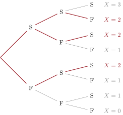
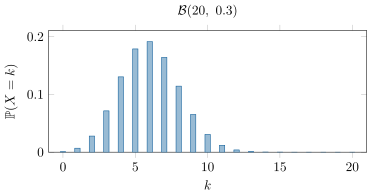
Repeat a Bernoulli trial $n$ times independently, and let $X$ be the total number of successes. The distribution of $X$ is the binomial distribution $\mathcal B(n, p)$ .

Three Bernoulli trials: exactly 32 = 3 of the 23 paths give two successes (red), each with probability p2(1-p), so (X = 2) = 3p2(1-p). — Three Bernoulli trials: exactly $\binom{3}{2} = 3$ of the $2^3$ paths give two successes (red), each with probability $p^2(1-p)$ , so $\P(X = 2) = 3p^2(1-p)$ .

Theorem 33.8

If $X \sim \mathcal B(n, p)$ , then for $0 \leq k \leq n$ :

\P(X = k) = \binom{n}{k} p^k (1-p)^{n-k},

and

\E(X) = np, \qquad \V(X) = np(1-p) .

Proof. A specified sequence of outcomes with $k$ successes and $n-k$ failures has probability $p^k(1-p)^{n-k}$ by independence; the number of such sequences is the number of ways to place the $k$ successes among the $n$ trials, namely $\binom nk$ (Chapter 27). Summing over the sequences gives the formula — and the binomial theorem confirms $\sum_k \P(X = k) = (p + q)^n = 1$ .

For the expectation, using $k\binom nk = n\binom{n-1}{k-1}$ (Exercise 27.7):

\E(X) = \sum_{k=1}^{n} k\binom nk p^k q^{n-k} = np\sum_{k=1}^{n} \binom{n-1}{k-1} p^{k-1} q^{(n-1)-(k-1)} = np\,(p + q)^{n-1} = np .

The variance formula is proved similarly with the identity $k(k-1)\binom nk = n(n-1)\binom{n-2}{k-2}$ , giving $\E(X(X-1)) = n(n-1)p^2$ , whence $\V(X) = n(n-1)p^2 + np - (np)^2 = np(1-p)$ . (A structural proof — the variance of a sum of independent variables — comes with Theorem 34.4.) ∎

The distribution B(20, 0.3): mean np = 6, standard deviation √npq 2.05. — The distribution $\mathcal B(20, 0.3)$ : mean $np = 6$ , standard deviation $\sqrt{npq} \approx 2.05$ .

Method 33.9 (Recognizing a binomial situation)

Check the three ingredients before writing $X \sim \mathcal B(n,p)$ : a fixed number $n$ of trials; two outcomes per trial with the same success probability $p$ ; independence of trials (sampling with replacement, or from a large population). Then use

\P(X \geq 1) = 1 - (1-p)^n

for “at least one success”, and a calculator or cumulative tables for general $\P(X \leq k)$ .

Example 33.10

How many times must one roll a die to have at least a $99\%$ chance of rolling a six? With $X \sim \mathcal B\left(n, \frac16\right)$ : $\P(X \geq 1) = 1 - \left(\frac56\right)^n \geq 0.99$ means $\left(\frac56\right)^n \leq 0.01$ , i.e. $n \geq \frac{\ln 0.01}{\ln(5/6)} \approx 25.3$ : from $n = 26$ rolls on.

33.3 Exercises

Exercise 33.1 ★

A random variable $X$ takes the values $-1, 0, 2, 5$ with probabilities $0.3, 0.2, 0.4, 0.1$ . Compute $\E(X)$ , $\V(X)$ and $\sigma(X)$ .

Solution

Solution of Exercise 33.1.

$\E(X) = -0.3 + 0 + 0.8 + 0.5 = 1$ . $\E(X^2) = 0.3 \times 1 + 0 + 0.4\times4 + 0.1\times25 = 4.4$ , so by König–Huygens $\V(X) = 4.4 - 1 = 3.4$ and $\sigma(X) = \sqrt{3.4} \approx 1.84$ .

Exercise 33.2 ★

A multiple-choice test has $10$ questions, each with $4$ choices, one of which is correct. A student answers uniformly at random, independently. Let $X$ be the number of correct answers.

Give the distribution of $X$ , $\E(X)$ and $\sigma(X)$ .
Compute $\P(X = 0)$ , $\P(X = 5)$ and $\P(X \geq 1)$ .

Solution

Solution of Exercise 33.2.

1. The $10$ questions are independent Bernoulli trials with $p = \frac14$ : $X \sim \mathcal B\left(10, \frac14\right)$ , $\E(X) = 2.5$ , $\sigma(X) = \sqrt{10 \times \frac14 \times \frac34} = \sqrt{1.875} \approx 1.37$ .

2. $\P(X = 0) = \left(\frac34\right)^{10} \approx 0.056$ ;

\P(X = 5) = \binom{10}{5}\left(\frac14\right)^5\left(\frac34\right)^5 \approx 0.058; \quad \P(X \geq 1) = 1 - \left(\tfrac34\right)^{10} \approx 0.944 .

Exercise 33.3 ★

An insurance company insures $n = 400$ clients; each files a claim during the year with probability $p = 0.05$ , independently. Let $X$ be the number of claims. Identify the distribution of $X$ and compute its expectation and standard deviation.

Solution

Solution of Exercise 33.3.

Independent identical trials: $X \sim \mathcal B(400,\ 0.05)$ , so $\E(X) = 20$ claims and

\sigma(X) = \sqrt{400 \times 0.05 \times 0.95} = \sqrt{19} \approx 4.4 .

Exercise 33.4 ★★

In the game of Example 33.5, the organizer wants a fair game ( $\E(G) = 0$ ) by changing the entry price $c$ . Find $c$ . Compute the variance of the gain for this fair version; is “fair” the same as “riskless”?

Solution

Solution of Exercise 33.4.

The payment $P$ received satisfies $\E(P) = \frac{5 + 6}{6} = \frac{11}{6}$ , so the fair price is $c = \frac{11}{6} \approx 1.83$ euros. The fair gain $G = P - \frac{11}6$ takes values $-\frac{11}{6}, \frac{19}{6}, \frac{25}{6}$ with probabilities $\frac46, \frac16, \frac16$ :

\V(G) = \E(G^2) = \frac{4 \times 121 + 361 + 625}{6 \times 36} = \frac{1470}{216} = \frac{245}{36} \approx 6.8, \qquad \sigma(G) \approx 2.6 .

A fair game has zero average gain but its outcomes still fluctuate: fair is not riskless.

Exercise 33.5 ★★

A basketball player scores free throws with probability $0.7$ . She shoots $8$ times (independent shots). Compute the probability that she scores: exactly $6$ ; at least $6$ ; at least once. What is the most probable number of scores?

Solution

Solution of Exercise 33.5.

$X \sim \mathcal B(8,\ 0.7)$ .

\P(X = 6) = \binom86 (0.7)^6(0.3)^2 \approx 0.296 ;

\P(X \geq 6) = \P(6) + \P(7) + \P(8) \approx 0.296 + 8(0.7)^7(0.3) + (0.7)^8 \approx 0.296 + 0.198 + 0.058 = 0.552 ;

$\P(X \geq 1) = 1 - (0.3)^8 \approx 0.99993$ . Mode: $(n+1)p = 6.3$ , so the most probable value is $k^* = 6$ (Exercise 33.7).

Exercise 33.6 ★★

An airline knows that each booked passenger shows up with probability $0.9$ , independently. A flight has $100$ seats and the airline sells $104$ tickets. Express, using a binomial distribution, the probability that more passengers show up than there are seats, and bound it numerically using a calculator (give the exact expression).

Solution

Solution of Exercise 33.6.

The number of passengers showing up is $X \sim \mathcal B(104,\ 0.9)$ ; the flight is overbooked when $X \geq 101$ :

\P(X \geq 101) = \sum_{k=101}^{104}\binom{104}{k}(0.9)^k(0.1)^{104-k} \approx 0.006 .

Selling $4\%$ more tickets than seats causes an incident on only about $0.6\%$ of flights — the economics behind overbooking.

Exercise 33.7 ★★

Let $X \sim \mathcal B(n, p)$ . Show that

\frac{\P(X = k+1)}{\P(X = k)} = \frac{n-k}{k+1}\cdot\frac{p}{1-p},

and deduce that the distribution increases up to $k^* = \floor{(n+1)p}$ and decreases afterwards (the mode of the binomial).

Solution

Solution of Exercise 33.7.

\frac{\P(X = k+1)}{\P(X = k)} = \frac{\binom{n}{k+1}}{\binom nk}\cdot\frac{p}{1-p} = \frac{n - k}{k + 1}\cdot\frac{p}{1-p},

using $\binom{n}{k+1} = \binom nk \frac{n-k}{k+1}$ . This ratio is $\geq 1$ iff $(n-k)p \geq (k+1)(1-p)$ iff $np - k p \geq k - kp + 1 - p$ iff $k \leq (n+1)p - 1$ . So the probabilities increase strictly while $k + 1 \leq (n+1)p$ and decrease afterwards: the maximum is attained at $k^* = \floor{(n+1)p}$ (shared with $k^* - 1$ when $(n+1)p$ is an integer).

Exercise 33.8 ★★★

(Saint Petersburg, tamed.) A fair coin is tossed until heads appears, but at most $10$ times. Let $N$ be the number of tosses used, and the player receives $2^N$ euros if heads appeared, $0$ otherwise.

Give the distribution of $N$ restricted to the winning outcomes: $\P(\text{heads first at toss } k) = 2^{-k}$ for $1 \leq k \leq 10$ , and check the total probability of winning.
Compute the expected payoff. What would it become without the cap of $10$ tosses?

Solution

Solution of Exercise 33.8.

1. Heads first at toss $k$ means $k-1$ tails then heads: probability $\left(\frac12\right)^{k-1}\cdot\frac12 = 2^{-k}$ , for $1 \leq k \leq 10$ . Total winning probability $\sum_{k=1}^{10} 2^{-k} = 1 - 2^{-10} = \frac{1023}{1024}$ (the game is lost only on ten consecutive tails).

2. Expected payoff:

\sum_{k=1}^{10} 2^k \cdot 2^{-k} = \sum_{k=1}^{10} 1 = 10 \text{ euros}.

Without the cap, the sum $\sum_{k\geq1} 1$ diverges: the expected payoff is infinite, although the game almost always pays a small amount — the famous Saint Petersburg paradox, showing that expectation alone does not measure the value of a game.

33.4 Problem: The overbooked flight

Problem 33.1

Weekend problem — airlines sell more seats than they have, factories accept lots they barely inspected, and the binomial distribution referees both

An airline with $100$ seats happily sells $105$ tickets: about $10\,\%$ of passengers never show up, and empty seats earn nothing. How far can the airline push before bumped passengers eat the profit? The binomial distribution (Theorem 33.8) answers to the decimal — and the same machinery inspects factory lots, prices raffles, and keeps insurers solvent. Decisions under repetition: this is the binomial’s day job.

Part I — Fluency.

Give the full distribution table of the number $X$ of sixes in three rolls of a die.
Compute $\E(X)$ and $V(X)$ (Definition 33.2).
A stall charges $1$ euro for three rolls and pays $2$ euros per six obtained. Compute the expected gain: fair game?
Checklist practice (Method 33.9): is the number of hearts in $5$ cards drawn without replacement binomial? With replacement? Justify.
For $X \sim \mathcal B(20,\ 0.3)$ : give $\E(X)$ and $\sigma(X)$ , then $\E(S)$ and $\sigma(S)$ for the score $S = 5X - 10$ (Proposition 33.4).

Part II — The overbooked flight. Seats: $100$ . Tickets sold: $105$ . Each ticket-holder shows up with probability $0.9$ , independently; let $X$ be the number who show.

Model: justify $X \sim \mathcal B(105,\ 0.9)$ with the checklist — and confess the model’s weakest point (are no-shows really independent? think groups and storms).
Compute $\E(X)$ and $\sigma(X)$ .
Bumping occurs when $X \geq 101$ : write $\P(X \geq 101)$ as an explicit sum of five binomial terms.
Evaluate the sum (calculator): what fraction of flights sees at least one bumped passenger?
Money: the five extra tickets bring $5 \times 200 = 1\,000$ euros; each bumped passenger costs $800$ euros in compensation. Compute the expected number of bumped passengers, $\sum_{k=101}^{105} (k - 100)\,\P(X = k)$ , the expected compensation, and the verdict on the policy.
Design: the regulator tolerates $\P(\text{bumping}) < 5\,\%$ . By testing $n = 105, 106, 107, \dots$ tickets, find the largest allowed $n$ .
The bell shortcut: for $n = 105$ , compute the z-score of the bumping threshold, $z = \frac{100.5 - \E(X)}{\sigma(X)}$ , and compare the crude “about $2\sigma$ , so roughly $2$ – $3\,\%$ in the upper tail” estimate with your exact answer. (The curve behind this shortcut is the next chapters’ star.)

Part III — The factory gate. A lot of parts is accepted if a sample of $20$ contains at most one defective part.

If the true defect rate is $2\,\%$ (an honest lot), compute the probability of acceptance.
If the rate is $10\,\%$ (a bad lot), compute it again.
Name the two risks of the procedure (the honest lot rejected; the bad lot accepted), read their values from questions 13–14, and say what single change improves both at once — at what cost.
Behind the improvement: show that the observed defect frequency $\frac Xn$ in a sample of size $n$ has standard deviation $\sqrt{\frac{p(1-p)}{n}}$ , and conclude how precision scales with sample size (an old friend: the $\frac{1}{\sqrt n}$ of grade 10).

Part IV — Games, raffles, reserves.

The capped Saint Petersburg game of Exercise 33.8 has expected payoff $10$ euros. Contrast in one paragraph with the uncapped paradox met in Problem 18.1: what exactly does the cap tame, and what price would now be fair?
A charity raffle sells $200$ tickets at $2$ euros; prizes: one $100$ -euro and two $50$ -euro baskets. Compute a ticket’s expected gain and the raffle’s margin; compare with European roulette’s house margin of $\frac{1}{37} \approx 2.7\,\%$ . Why does the raffle get away with it?
An insurer holds $1\,000$ independent policies: claim probability $0.01$ each, claim size $10\,000$ euros, premium $130$ euros. Compute the expected annual profit and the standard deviation of total claims. Compare the two numbers: what does the comparison force real insurers to hold?
Finale — the binomial as decision referee: the recognition checklist; the compass $\E \pm \sigma$ ; tail probabilities as the price of risk; and the two standing caveats (independence is a modeling claim, and rare tails, not means, cause ruin). One sentence each, with the pointer: the law of large numbers and the bell curve, next chapters, complete the referee’s rulebook.

Solution

Solution of Problem 33.1.

1. $X \sim \mathcal B\!\left(3, \frac16\right)$ : $\P(X = 0) = \frac{125}{216}$ , $\P(X = 1) = \frac{75}{216}$ , $\P(X = 2) = \frac{15}{216}$ , $\P(X = 3) = \frac{1}{216}$ .

2. $\E(X) = 3 \times \frac16 = \frac12$ ; $V(X) = 3 \times \frac16 \times \frac56 = \frac{5}{12}$ .

3. Expected payout $2\,\E(X) = 1$ euro against a $1$ -euro stake: gain $0$ — exactly fair (a rarity).

4. Without replacement the draws are dependent (the second card’s chances depend on the first): not binomial — the checklist’s independence box fails. With replacement: fixed $n = 5$ , constant $p = \frac14$ , independent draws: binomial.

5. $\E(X) = 6$ , $\sigma(X) = \sqrt{4.2} \approx 2.05$ . $\E(S) = 5 \times 6 - 10 = 20$ ; $\sigma(S) = 5\sigma(X) \approx 10.25$ .

6. Fixed $n = 105$ trials (the tickets), each a show/no-show with the same $p = 0.9$ , assumed independent: binomial. The confession: families miss flights together and storms empty whole planes — independence is the model’s leap of faith, and correlated no-shows make the tails fatter than the binomial promises.

7. $\E(X) = 94.5$ ; $\sigma(X) = \sqrt{105 \times 0.9 \times 0.1} = \sqrt{9.45} \approx 3.07$ .

8. $\P(X \geq 101) = \sum_{k=101}^{105} \binom{105}{k} 0.9^k\, 0.1^{105 - k}$ .

9. $\approx 0.0167$ : about one flight in sixty bumps anyone at all.

10. $\E(\text{bumped}) \approx 0.023$ passengers per flight: expected compensation $\approx 19$ euros — against $1\,000$ euros of extra revenue. Overbooking by five is overwhelmingly profitable; hence every airline does it.

11. From the table of tail probabilities: $n = 105$ : $1.7\,\%$ ; $n = 106$ : $4.0\,\%$ ; $n = 107$ : $8.1\,\%$ . The largest compliant sale is $n = 106$ tickets.

12. $z = \frac{100.5 - 94.5}{3.07} \approx 1.95$ : the threshold sits two standard deviations above the mean, and the bell-curve rule of thumb (“upper $2\sigma$ tail $\approx 2.5\,\%$ ”) lands close to the exact $1.7\,\%$ — the smooth curve shadowing the binomial is the coming chapters’ protagonist.

13. $0.98^{20} + 20 \times 0.02 \times 0.98^{19} \approx 0.94$ : the honest lot passes $94\,\%$ of the time.

14. $0.9^{20} + 20 \times 0.1 \times 0.9^{19} \approx 0.39$ : the bad lot still sneaks through $39\,\%$ of the time.

15. Producer’s risk: a good lot rejected ( $\approx 6\,\%$ ); consumer’s risk: a bad lot accepted ( $\approx 39\,\%$ ). A larger sample (with a proportional acceptance threshold) shrinks both — at the cost of more inspection: quality has a budget line.

16. $V\!\left(\frac Xn\right) = \frac{V(X)}{n^2} = \frac{np(1-p)}{n^2} = \frac{p(1-p)}{n}$ : standard deviation $\sqrt{\frac{p(1-p)}{n}}$ . Quadruple the sample, halve the noise: the $\frac{1}{\sqrt n}$ law of grade 10’s fluctuation intervals, now derived.

17. The cap bounds the payout at $2^{10} = 1024$ euros, so each of the ten rounds contributes exactly $1$ euro of expectation: $\E = 10$ . The uncapped game’s infinite expectation came entirely from astronomically rare, astronomically large payoffs; capping confesses that no bank pays $2^{50}$ euros. A fair ticket price for the capped game: $10$ euros — and suddenly nobody is paradoxed.

18. Expected prize money per ticket: $\frac{100 + 2 \times 50}{200} = 1$ euro against a $2$ -euro ticket: margin $50\,\%$ — eighteen times roulette’s $2.7\,\%$ . The raffle survives because its players are knowingly donating: the “loss” is the point.

19. Expected claims: $1\,000 \times 0.01 \times 10\,000 = 100\,000$ ; premiums $130\,000$ : expected profit $30\,000$ euros. Standard deviation of total claims: $10\,000 \times \sqrt{1\,000 \times 0.01 \times 0.99} \approx 31\,500$ euros — one ordinary bad year devours the whole expected profit. Hence capital reserves, reinsurance, and portfolios far larger than a thousand policies: insurers live off the law of large numbers and keep reserves against its slowness.

20. Checklist first — fixed $n$ , same $p$ , independence claimed — or no binomial at all. Then navigate by $\E \pm \sigma$ : means locate, deviations warn. Then price the tails: bumping, bad lots, ruinous years all live beyond $2\sigma$ . Caveats: independence is the modeler’s promise, not the world’s; and expectation ignores exactly what destroys you. The rulebook’s missing pages — how fast frequencies settle, and what shape the fluctuations take — are the next two chapters.