High School Mathematics · Grades 10–12

8Descriptive Statistics

Statistics summarizes a large collection of numbers — grades, salaries, temperatures — by a few well-chosen indicators. This chapter introduces the two families of indicators: those locating the center of the data (mean, median) and those measuring its spread (range, quartiles). A deeper treatment, including the standard deviation, comes in Chapter 17.

8.1 Data and frequencies

Definition 8.1 (Statistical series)

A statistical series is a list of values $x_1, x_2, \dots, x_N$ observed on a population of size $N$ . When a value $x$ appears $n$ times, $n$ is its count and the quotient

f = \frac{n}{N}

is its frequency (often expressed as a percentage). The frequencies of all values add up to $1$ .

Example 8.2

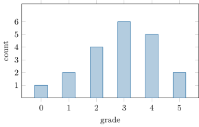
The grades of $20$ students on a $5$ -point quiz:

grade $x$	$0$	$1$	$2$	$3$	$4$	$5$
count $n$	$1$	$2$	$4$	$6$	$5$	$2$
frequency $f$	$0.05$	$0.10$	$0.20$	$0.30$	$0.25$	$0.10$

Check: $1 + 2 + 4 + 6 + 5 + 2 = 20$ and the frequencies sum to $1$ .

The bar chart of the quiz grades: one bar per value, with height equal to the count.

8.2 Measures of center

Definition 8.3 (Mean)

The mean of the series is

\bar x = \frac{x_1 + x_2 + \dots + x_N}{N}.

If the values $v_1, \dots, v_k$ appear with counts $n_1, \dots, n_k$ , the same number is computed as the weighted mean

\bar x = \frac{n_1 v_1 + n_2 v_2 + \dots + n_k v_k}{n_1 + n_2 + \dots + n_k}.

Example 8.4

For the quiz of Example 8.2:

\bar x = \frac{1 \times 0 + 2 \times 1 + 4 \times 2 + 6 \times 3 + 5 \times 4 + 2 \times 5}{20} = \frac{0 + 2 + 8 + 18 + 20 + 10}{20} = \frac{58}{20} = 2.9 .

Definition 8.5 (Median)

The median is a value that splits the sorted series in two halves: at least half the values are $\leq$ the median, and at least half are $\geq$ it. In practice, sort the $N$ values;

if $N$ is odd, the median is the middle value, in position $\frac{N+1}{2}$ ;
if $N$ is even, take the midpoint of the two middle values, in positions $\frac N2$ and $\frac N2 + 1$ .

Example 8.6

Sorted series of $7$ house prices (in thousands): $120$ , $150$ , $160$ , $180$ , $210$ , $240$ , $900$ . The median is the $4$ th value, $180$ . The mean is $\frac{1960}{7} = 280$ — larger than $6$ of the $7$ prices! One extreme value ( $900$ ) pulls the mean far more than the median: the median is robust, the mean is not.

8.3 Measures of spread

Definition 8.7 (Range, quartiles)

For a sorted series:

the range is the difference between the largest and smallest values;
the first quartile $Q_1$ is the smallest value such that at least a quarter ( $25\%$ ) of the values are $\leq Q_1$ ; the third quartile $Q_3$ is the smallest value such that at least three quarters ( $75\%$ ) of the values are $\leq Q_3$ ;
the interquartile range $Q_3 - Q_1$ measures the spread of the central half of the data.

Method 8.8 (Finding the quartiles)

For a series of $N$ sorted values:

compute $\frac N4$ ; if it is not an integer round it up to the next integer; $Q_1$ is the value in that position;
compute $\frac{3N}{4}$ ; round up if needed; $Q_3$ is the value in that position.

Example 8.9

Take the $11$ sorted values

2,\ 3,\ 5,\ 5,\ 6,\ 7,\ 8,\ 9,\ 9,\ 10,\ 12 .

Median: position $\frac{11+1}{2} = 6$ , so the median is $7$ . $Q_1$ : $\frac{11}{4} = 2.75$ , round up to $3$ ; the $3$ rd value is $5$ . $Q_3$ : $\frac{33}{4} = 8.25$ , round up to $9$ ; the $9$ th value is $9$ . Range: $12 - 2 = 10$ ; interquartile range: $9 - 5 = 4$ .

The box plot of : the box spans the interquartile interval [Q_1, Q_3] and contains the central half of the data; the whiskers reach the extreme values. — The box plot of Example 8.9: the box spans the interquartile interval $\intcc{Q_1}{Q_3}$ and contains the central half of the data; the whiskers reach the extreme values.

Example 8.10 (Comparing two groups)

Two classes take the same test (scores out of $20$ ):

	median	$Q_1$	$Q_3$
class A	$12$	$10$	$14$
class B	$12$	$6$	$17$

Same median, very different spreads: class A is homogeneous (half its scores in $\intcc{10}{14}$ ), class B is heterogeneous (its central half spans $\intcc{6}{17}$ ). Indicators of center alone never tell the whole story.

Remark 8.11

Neither the mean nor the median is “better”: the mean uses every value (and is needed to compute totals), the median resists extreme values. A serious summary of a series gives at least one indicator of center and one of spread.

8.4 Exercises

Exercise 8.1 ★

Here are the numbers of books read in a year by $15$ students:

0,\ 1,\ 1,\ 2,\ 2,\ 2,\ 3,\ 3,\ 4,\ 4,\ 5,\ 6,\ 7,\ 8,\ 12 .

Compute the mean, the median and the range of this series.

Solution

Solution of Exercise 8.1.

Sum: $0+1+1+2+2+2+3+3+4+4+5+6+7+8+12 = 60$ , so the mean is $\frac{60}{15} = 4$ . The series is already sorted and $N = 15$ is odd: the median is the $8$ th value, $3$ . Range: $12 - 0 = 12$ .

Exercise 8.2 ★

A die was rolled $50$ times:

outcome	$1$	$2$	$3$	$4$	$5$	$6$
count	$7$	$9$	$8$	$10$	$6$	$10$

Compute the frequency of each outcome and the mean outcome.

Solution

Solution of Exercise 8.2.

Frequencies: $\frac{7}{50} = 0.14$ , $\frac{9}{50} = 0.18$ , $\frac{8}{50} = 0.16$ , $\frac{10}{50} = 0.20$ , $\frac{6}{50} = 0.12$ , $\frac{10}{50} = 0.20$ (sum $1$ ). Mean outcome:

\bar x = \frac{7 \times 1 + 9 \times 2 + 8 \times 3 + 10 \times 4 + 6 \times 5 + 10 \times 6}{50} = \frac{7 + 18 + 24 + 40 + 30 + 60}{50} = \frac{179}{50} = 3.58 .

Exercise 8.3 ★

Find the median, $Q_1$ and $Q_3$ of the sorted series

1,\ 2,\ 4,\ 4,\ 5,\ 6,\ 6,\ 7,\ 8,\ 9,\ 9,\ 11 \qquad (N = 12),

and draw the corresponding box plot.

Solution

Solution of Exercise 8.3.

$N = 12$ (even): the median is the midpoint of the $6$ th and $7$ th values, both equal to $6$ : median $6$ .

$Q_1$ : $\frac{12}{4} = 3$ , so $Q_1$ is the $3$ rd value: $4$ .

$Q_3$ : $\frac{3 \times 12}{4} = 9$ , so $Q_3$ is the $9$ th value: $8$ .

Box plot: box from $4$ to $8$ with the median bar at $6$ , whiskers from $1$ to $11$ .

Exercise 8.4 ★

The mean of $24$ test scores is $11.5$ . A $25$ th student takes the test and scores $19$ . What is the new mean of the class?

Solution

Solution of Exercise 8.4.

The $24$ scores total $24 \times 11.5 = 276$ . With the new score the total is $276 + 19 = 295$ for $25$ students: new mean $\frac{295}{25} = 11.8$ .

Exercise 8.5 ★★

A student has a mean of $12$ after $5$ tests, all with the same weight. What score on the $6$ th test would raise the mean to $13$ ? Is a mean of $14$ reachable (scores are out of $20$ )?

Solution

Solution of Exercise 8.5.

Current total: $5 \times 12 = 60$ . A mean of $13$ over $6$ tests requires a total of $78$ , so the $6$ th score must be $78 - 60 = 18$ . A mean of $14$ would require $84 - 60 = 24 > 20$ : not reachable.

Exercise 8.6 ★★

Invent a series of $7$ nonnegative values whose median is $10$ and whose mean is larger than $20$ ; then one whose median is $10$ and whose mean is smaller than $6$ . Why can the mean of such a series never be smaller than $\frac{40}{7}$ ? What do these examples show?

Solution

Solution of Exercise 8.6.

Mean larger than $20$ : for instance $1,\ 2,\ 3,\ 10,\ 40,\ 50,\ 60$ — median $10$ (the $4$ th sorted value), mean $\frac{166}{7} \approx 23.7$ .

Mean smaller than $6$ : for instance $0,\ 0,\ 0,\ 10,\ 10,\ 10,\ 10$ — median $10$ , mean $\frac{40}{7} \approx 5.7$ .

The mean cannot go below $\frac{40}{7}$ : for the median (the $4$ th sorted value) to be $10$ , the values in positions $4$ to $7$ must all be $\geq 10$ , so the total is at least $40$ and the mean at least $\frac{40}{7}$ — the second example is extremal.

These examples show that the mean and the median are largely independent: knowing one says little about the other, which is why a good summary reports both.

Exercise 8.7 ★★

In a company, the $9$ employees earn $1800$ each per month and the director earns $12000$ .

Compute the mean and the median salary.
Which indicator best describes a “typical” salary here? Why?

Solution

Solution of Exercise 8.7.

1. Mean: $\frac{9 \times 1800 + 12000}{10} = \frac{16200 + 12000}{10} = 2820$ . Median: sorted, the $10$ salaries are nine values $1800$ then $12000$ ; the median is the midpoint of the $5$ th and $6$ th values, both $1800$ : median $1800$ .

2. The median ( $1800$ ) describes the typical salary: it is what $9$ employees out of $10$ actually earn. The mean ( $2820$ ) is pulled up by the single high salary and matches nobody’s payslip.

Exercise 8.8 ★★

A class of $12$ boys has a mean height of $168$ cm; the $18$ girls of the same class have a mean height of $163$ cm. Compute the mean height of the whole class. (Careful: it is not the midpoint of $168$ and $163$ — weight the means by the group sizes.)

Solution

Solution of Exercise 8.8.

Total height: $12 \times 168 + 18 \times 163 = 2016 + 2934 = 4950$ cm for $30$ students, so the mean is $\frac{4950}{30} = 165$ cm. It is closer to the girls’ mean because they are more numerous (weighted mean, weights $12$ and $18$ ).

Exercise 8.9 ★★★

A series of $N$ values $x_1, \dots, x_N$ has mean $\bar x$ . Each value is transformed into $y_i = a x_i + b$ for fixed numbers $a$ and $b$ .

Show that the mean of the new series is $a \bar x + b$ .
The temperatures of a week, in degrees Celsius, have mean $20$ . What is their mean in degrees Fahrenheit ( $F = 1.8\,C + 32$ )?

Solution

Solution of Exercise 8.9.

1. The new mean is

\bar y = \frac{y_1 + \dots + y_N}{N} = \frac{(a x_1 + b) + \dots + (a x_N + b)}{N} = \frac{a(x_1 + \dots + x_N) + Nb}{N} = a \bar x + b .

2. With $a = 1.8$ and $b = 32$ : mean $1.8 \times 20 + 32 = 68$ degrees Fahrenheit.

8.5 Problem: The average person does not exist

Problem 8.1

Weekend problem — mean against median: outliers, grading curves, the warehouse on the road, and the cockpit designed for nobody

In 1950 the US Air Force measured $4\,000$ pilots on ten body dimensions and built the cockpit for the average man. It fitted — as one lieutenant discovered by counting — essentially nobody. Statistics summarizes crowds with single numbers, and each summary tells the truth about something and lies about something else. This problem takes the mean and the median (Definition 8.3, Definition 8.5) to court, lets each show what it is best at, and closes the cockpit case.

Part I — Two summaries on trial.

A street sells seven houses, in thousands of euros: $200$ , $210$ , $220$ , $230$ , $240$ , $250$ — and one mansion at $1\,200$ . Compute the mean and the median price. Which number describes “a house in this street”?
Remove the mansion and recompute both. By how much did each summary move? State the moral about outliers.
A census table: out of $100$ families, $20$ have no child, $25$ have one, $30$ have two, $15$ have three, $10$ have four. Compute the mean number of children. No family “has $1.7$ children” — so what real quantity does the mean encode? (Multiply it by $100$ .)
For the fifteen marks $4, 6, 7, 8, 9, 10, 10, 11, 12, 12, 13, 14, 15, 17, 19$ : find the median and the quartiles $Q_1$ , $Q_3$ (Method 8.8).
For the same series, give the range and the interquartile range. What does each measure?

Part II — Grading curves and merged classes.

From Exercise 8.9: shifting every value by $+b$ shifts mean, median and quartiles by $+b$ ; scaling by $a$ scales them by $a$ . What happens to the range and the interquartile range under a shift? Under a scaling? Justify.
A test has mean $9$ (out of $20$ ) and the teacher wants mean $12$ . Two curves are proposed: add $3$ points to everyone, or multiply every mark by $\frac43$ . Compute the fate of a student at $6$ and one at $18$ under each curve. Which curve favors whom — and which has a ceiling problem?
Class A ( $20$ students) has mean $12$ ; class B ( $30$ students) has mean $10$ . Compute the mean of the $50$ students together, and explain why it is not $11$ (the weighted-average lesson of the harmonic-mean weekend problem of the Middle School volume, in the classroom).
Show that medians refuse this game: compute the medians of $A = \{1, 2, 3\}$ and $B = \{0, 10\}$ , then the median of the merged list, and compare with the size-weighted average of the two medians.
Figure skating: five judges score $5.2$ , $5.3$ , $5.4$ , $5.5$ , $9.9$ . Compute the mean, the median, and the trimmed mean (drop the lowest and highest, average the rest). Why do most judged sports trim?

Part III — Reading distributions.

Two factories both produce bolts of mean length $50$ mm. Factory A: $Q_1 = 49.9$ , $Q_3 = 50.1$ ; factory B: $Q_1 = 48$ , $Q_3 = 52$ . You need interchangeable bolts: which factory, and which statistic decided?
At a clinic, the median wait is $10$ minutes but the mean wait is $25$ . What shape of data does this pair betray? Construct a five-value dataset with exactly this median and mean.
“Your baby is at the 75th percentile for height” — what does that sentence mean? And can every child of a town be “above average”? Above the median? Explain the difference.
Class A: min $4$ , $Q_1\,8$ , median $11$ , $Q_3\,13$ , max $17$ . Class B: min $2$ , $Q_1\,9$ , median $11$ , $Q_3\,12$ , max $19$ . Compare: typical mark, homogeneity of the middle half, wildness of the extremes.
The journalist’s checklist: a headline says “average salary at TechCorp: $5\,000$ euros”. List the three questions this problem has taught you to ask before believing the headline says anything about a typical employee.

Part IV — The cockpit case.

Build your own evidence: construct five house prices with mean $300$ and median $200$ (thousands of euros).
The mean is the balance point: prove from the definition that the deviations from the mean always cancel, $\sum (x_i - \bar x) = 0$ , and verify it on your dataset of question 16.
The median is the errand-minimizer: shops sit at kilometers $1$ , $3$ , $4$ , $9$ , $13$ of a road, and a warehouse must minimize the total distance to the five shops. Compute that total for a warehouse at the median ( $4$ ), at the mean ( $6$ ), and at $5$ . Who wins? (This is general: the median minimizes total absolute distance — test any other spot.)
The cockpit, resolved: suppose a pilot has a $30\,\%$ chance of being “close to average” on one body dimension, independently across $10$ dimensions. Estimate the chance of being close to average on all ten — and reconcile the result with what the lieutenant found in $4\,000$ pilots. What did the Air Force build instead of the average cockpit?
Finale — the user’s guide, one line each: when totals are what matters (a budget, a harvest), use the …; when the typical individual matters (salaries, waiting times), use the …; when fairness of spread matters, report the …; when contamination threatens, use the …. Close the case with the problem’s title.

Solution

Solution of Problem 8.1.

1. Mean: $\frac{2\,550}{7} \approx 364$ thousand euros; median: the fourth of the seven ordered prices, $230$ . The median describes the street — six of the seven houses cost nowhere near $364$ .

2. Without the mansion: mean $\frac{1\,350}{6} = 225$ , median $\frac{220 + 230}{2} = 225$ . The mean fell by about $139$ ; the median by $5$ . One extreme value can drag the mean anywhere; the median barely notices — it is robust.

3. Mean $= \frac{0 \times 20 + 1 \times 25 + 2 \times 30 + 3 \times 15 + 4 \times 10}{100} = \frac{170}{100} = 1.7$ . No family has $1.7$ children, but $1.7 \times 100 = 170$ is the exact total number of children: the mean encodes the total, redistributed equally — its true talent.

4. $N = 15$ : median $=$ 8th value $= 11$ ; $Q_1 =$ 4th value $= 8$ ; $Q_3 =$ 12th value $= 14$ .

5. Range $19 - 4 = 15$ : the full spread, extremes included. Interquartile range $14 - 8 = 6$ : the width of the middle half — spread without the extremes’ noise.

6. A shift $+b$ moves every value, so differences of values — range, IQR — are unchanged: $(x_i + b) - (x_j + b) = x_i - x_j$ . A scaling by $a$ multiplies all differences by $a$ : range and IQR are scaled by $\abs a$ .

7. Additive curve: $6 \to 9$ and $18 \to 21$ — the weak student gains $50\,\%$ , the strong one $17\,\%$ , and $21$ bursts the $20$ -point scale only mildly. Multiplicative: $6 \to 8$ and $18 \to 24$ — ratios preserved, but $24$ is impossible on a $20$ -scale: the ceiling problem. Additive curves flatter the bottom; multiplicative ones explode the top.

8. Total marks: $20 \times 12 + 30 \times 10 = 540$ , so the merged mean is $\frac{540}{50} = 10.8$ : class B’s thirty students outweigh class A’s twenty — means merge by weighted average, never by simple average.

9. Median of $A$ : $2$ ; of $B$ : $5$ . Merged list $\{0, 1, 2, 3, 10\}$ : median $2$ . The size-weighted average of the medians would be $\frac{3 \times 2 + 2 \times 5}{5} = 3.2 \neq 2$ : medians carry no total, so no merging formula exists — one must re-sort the whole list.

10. Mean: $\frac{31.3}{5} = 6.26$ . Median: $5.4$ . Trimmed mean: $\frac{5.3 + 5.4 + 5.5}{3} = 5.4$ . One enthusiastic (or corrupt) judge moved the mean by almost a point; the median and the trimmed mean shrugged — hence the trimming rules of judged sports.

11. Factory A: middle half within $0.2$ mm; factory B: within $4$ mm. Same mean, opposite reliability: buy from A. The interquartile range decided — means alone compare centers, never consistency.

12. Median far below mean betrays a long right tail: most waits short, a few catastrophic. Example: $\{5, 5, 10, 10, 95\}$ — median $10$ , mean $\frac{125}{5} = 25$ .

13. It means $75\,\%$ of babies of that age are shorter (and $25\,\%$ taller): a rank, not a size. “Every child above the mean” is impossible — if all values exceeded the mean, their average would exceed the mean, which is itself: contradiction. But almost all can be: one very short child can hold the mean below everyone else. Above the median: never more than half, by definition. Ranks cannot be flattered; averages can.

14. Typical mark: same, median $11$ for both. Homogeneity of the middle: B tighter (IQR $3$ against $5$ ). Extremes: B wilder (range $17$ against $13$ ). B is a class of similar students plus a few outliers; A is evenly spread.

15. (1) Is $5\,000$ the mean or the median — and may I have the median? (2) What is the spread (quartiles), so I know how typical “typical” is? (3) Who was counted — sample size and selection (the how-data-lies weekend problem of the Middle School volume’s poll lesson)?

16. For instance $100, 150, 200, 250, 800$ : median $200$ , mean $\frac{1\,500}{5} = 300$ .

17. $\sum (x_i - \bar x) = \sum x_i - N \bar x = N\bar x - N\bar x = 0$ . Check: $-200 - 150 - 100 - 50 + 500 = 0$ . The mean is the point where the deviations balance — the data’s center of gravity (the centroid weekend problem of the Middle School volume’s $G$ , in one dimension).

18. At the median $4$ : $3 + 1 + 0 + 5 + 9 = 18$ km. At the mean $6$ : $5 + 3 + 2 + 3 + 7 = 20$ km. At $5$ : $4 + 2 + 1 + 4 + 8 = 19$ km. The median wins — moving away from it always passes more shops than it approaches, so the total can only grow.

19. $0.3^{10} \approx 6 \times 10^{-6}$ : about six pilots per million. In $4\,000$ pilots the expected count is $0.02$ — zero, as lieutenant Daniels found. The Air Force stopped designing for the average man and made everything adjustable: seats, pedals, straps — design for the spread, not the center.

20. Totals: the mean. Typical individual: the median. Fairness of spread: the quartiles (and IQR). Contamination: the trimmed mean. And the closing line: the average person does not exist — but the median person almost does.