High School Mathematics · Grades 10–12

11Functions and Variations

This chapter organizes what one needs to know about functions before calculus: the small family of reference functions whose graphs must be known by heart, the precise meaning of increasing and decreasing, and how variations behave when functions are combined.

11.1 Functions and curves

Definition 11.1 (Function, domain, curve)

A function $f$ assigns to each number $x$ of a set $D \subseteq \R$ (its domain) exactly one number $f(x)$ . Its curve (or graph) is the set of points $\bigl(x, f(x)\bigr)$ for $x \in D$ .

Example 11.2

The formula $f(x) = \frac{\sqrt{x+2}}{x-1}$ requires $x + 2 \geq 0$ (for the square root) and $x \neq 1$ (nonzero denominator): the domain is $\intco{-2}{1} \cup \intoo{1}{+\infty}$ .

11.2 The reference functions

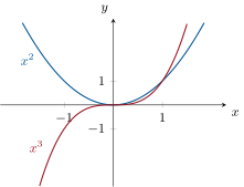
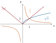
The following five functions and their curves must become reflexes.

Definition 11.3 (Reference functions)

x \mapsto x^2 \text{ (square)}, \quad x \mapsto x^3 \text{ (cube)}, \quad x \mapsto \sqrt{x}, \quad x \mapsto \frac{1}{x}, \quad x \mapsto \abs{x}.

Their domains are $\R$ , $\R$ , $\intco{0}{+\infty}$ , $\R \setminus \{0\}$ and $\R$ respectively. The curve of $x \mapsto \frac1x$ is a hyperbola.

The five reference curves: the parabola x2 and the cube x3 (left); √ x, x and the hyperbola 1x (right). — The five reference curves: the parabola $x^2$ and the cube $x^3$ (left); $\sqrt x$ , $\abs x$ and the hyperbola $\frac1x$ (right).

11.3 Variations on an interval

Definition 11.4 (Increasing, decreasing)

Let $f$ be defined on an interval $I$ . The function $f$ is increasing on $I$ if it preserves order:

\text{for all } u, v \in I: \quad u < v \implies f(u) \leq f(v),

and decreasing if it reverses order ( $u < v \implies f(u) \geq f(v)$ ). With strict inequalities on the right, $f$ is strictly increasing (resp. decreasing). A function that is increasing or decreasing on $I$ is monotonic on $I$ .

Method 11.5 (Proving a variation from the definition)

Take two arbitrary numbers $u < v$ in the interval, and determine the sign of the difference $f(v) - f(u)$ , usually by factoring it. If the sign is constant on the interval, conclude.

Proposition 11.6 (Variations of the reference functions)

$x^2$ is strictly decreasing on $\intoc{-\infty}{0}$ and strictly increasing on $\intco{0}{+\infty}$ .
$x^3$ is strictly increasing on $\R$ .
$\sqrt x$ is strictly increasing on $\intco{0}{+\infty}$ .
$\frac1x$ is strictly decreasing on $\intoo{-\infty}{0}$ and on $\intoo{0}{+\infty}$ (but not on their union).
$\abs x$ is strictly decreasing on $\intoc{-\infty}{0}$ and strictly increasing on $\intco{0}{+\infty}$ .

Proof. Let $u < v$ . We factor $f(v) - f(u)$ in each case.

1. $v^2 - u^2 = (v-u)(v+u)$ . On $\intco{0}{+\infty}$ : $v - u > 0$ and $v + u > 0$ (as $v > u \geq 0$ ), so $v^2 > u^2$ . On $\intoc{-\infty}{0}$ : $v + u < 0$ , so $v^2 < u^2$ .

2. $v^3 - u^3 = (v - u)(v^2 + uv + u^2)$ , and the second factor equals $\left(v + \frac u2\right)^2 + \frac{3u^2}{4} > 0$ unless $u = v = 0$ . Hence $v^3 > u^3$ whenever $v > u$ .

3. For $0 \leq u < v$ : $\sqrt v - \sqrt u = \frac{(\sqrt v - \sqrt u)(\sqrt v + \sqrt u)} {\sqrt v + \sqrt u} = \frac{v - u}{\sqrt v + \sqrt u} > 0$ .

4. For $0 < u < v$ : $\frac1v - \frac1u = \frac{u - v}{uv} < 0$ since $u - v < 0$ and $uv > 0$ ; same computation for $u < v < 0$ . On the union the claim fails: $-1 < 1$ but $\frac{1}{-1} = -1 < 1 = \frac11$ .

5. On $\intco{0}{+\infty}$ , $\abs x = x$ is strictly increasing; on $\intoc{-\infty}{0}$ , $\abs x = -x$ is strictly decreasing. ∎

Remark 11.7

Point 4 is a classic trap: “decreasing on $\intoo{-\infty}{0}$ and on $\intoo{0}{+\infty}$ ” is not the same as “decreasing on $\R \setminus \{0\}$ ”. Variations only make sense on intervals.

Example 11.8 (Comparing without computing)

Since $\sqrt x$ is strictly increasing, $\sqrt{7} < \sqrt{8}$ ; since $x^2$ is strictly decreasing on $\intoc{-\infty}{0}$ , $(-3)^2 > (-2)^2$ . Monotonicity turns comparisons of images into comparisons of arguments.

11.4 New functions from old

Proposition 11.9 (Transformations)

Let $u$ be a function defined on an interval $I$ and $k \in \R$ .

$u + k$ has the same variations as $u$ on $I$ ; its curve is that of $u$ shifted vertically by $k$ .
For $\lambda > 0$ , $\lambda u$ has the same variations as $u$ ; for $\lambda < 0$ , the variations are reversed.
If $u \geq 0$ on $I$ , then $\sqrt u$ has the same variations as $u$ .
If $u \neq 0$ and $u$ has constant sign on $I$ , then $\frac1u$ has the variations opposite to those of $u$ .

Proof. Let $u < v$ in $I$ (abusing notation, we compare $x$ -values $u < v$ ; write $s = u(x_1)$ , $t = u(x_2)$ for the images of $x_1 < x_2$ ).

1. $(u+k)(x_2) - (u+k)(x_1) = t - s$ : the difference of images is unchanged, so its sign is unchanged.

2. $\lambda t - \lambda s = \lambda(t - s)$ : the sign is kept if $\lambda > 0$ , flipped if $\lambda < 0$ .

3. If $u$ is increasing and $x_1 < x_2$ , then $0 \leq s \leq t$ , and $\sqrt{}$ being increasing (Proposition 11.6) gives $\sqrt s \leq \sqrt t$ . Same argument in the decreasing case.

4. If $u$ is increasing, $0 < s \leq t$ (or $s \leq t < 0$ ), then $\frac1s \geq \frac1t$ because $x \mapsto \frac1x$ is decreasing on each side of $0$ : the order is reversed. ∎

Example 11.10

Study $f(x) = \sqrt{x^2 + 1}$ on $\R$ . The inner function $u(x) = x^2 + 1$ is positive, decreasing on $\intoc{-\infty}{0}$ and increasing on $\intco{0}{+\infty}$ (a shifted square). By point 3, $f$ has the same variations: decreasing then increasing, with minimum $f(0) = 1$ .

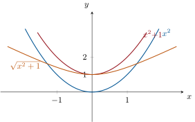
Transformations in action: shifting x2 up by 1 (red) keeps its variations; taking the square root (orange) keeps them again, as in . — Transformations in action: shifting $x^2$ up by $1$ (red) keeps its variations; taking the square root (orange) keeps them again, as in Example 11.10.

11.5 Even and odd functions

Definition 11.11 (Parity)

Let $f$ be defined on a domain $D$ symmetric about $0$ (i.e. $-x \in D$ whenever $x \in D$ ). The function $f$ is even if $f(-x) = f(x)$ for all $x \in D$ , and odd if $f(-x) = -f(x)$ for all $x \in D$ .

Proposition 11.12 (Geometric meaning)

The curve of an even function is symmetric about the $y$ -axis; the curve of an odd function is symmetric about the origin.

Proof. If $f$ is even and $(x, y)$ is on the curve (so $y = f(x)$ ), then $f(-x) = f(x) = y$ : the mirror point $(-x, y)$ is also on the curve. If $f$ is odd, $f(-x) = -y$ : the point $(-x, -y)$ , symmetric of $(x,y)$ about the origin, is on the curve. ∎

Example 11.13

$x^2$ and $\abs x$ are even; $x^3$ and $\frac1x$ are odd; $f(x) = x^2 + x$ is neither: $f(-1) = 0$ while $f(1) = 2$ , so $f(-1) \neq \pm f(1)$ . Parity halves the work: an even or odd function only needs to be studied on $\intco{0}{+\infty}$ .

11.6 Exercises

Exercise 11.1 ★

Give the domain of each function:

f(x) = \sqrt{3 - x}, \qquad g(x) = \frac{1}{x^2 - 4}, \qquad h(x) = \frac{\sqrt{x}}{x - 5} .

Solution

Solution of Exercise 11.1.

$f$ : need $3 - x \geq 0$ , domain $\intoc{-\infty}{3}$ .

$g$ : need $x^2 - 4 \neq 0$ , i.e. $x \neq \pm 2$ : domain $\R \setminus \{-2, 2\}$ .

$h$ : need $x \geq 0$ and $x \neq 5$ : domain $\intco{0}{5} \cup \intoo{5}{+\infty}$ .

Exercise 11.2 ★

Using the variations of the reference functions, compare without a calculator:

\sqrt{11} \text{ and } \sqrt{13}; \qquad (-2.1)^2 \text{ and } (-2.05)^2; \qquad \frac{1}{0.9} \text{ and } \frac{1}{1.1}; \qquad (-1.01)^3 \text{ and } (-0.99)^3 .

Solution

Solution of Exercise 11.2.

$\sqrt{11} < \sqrt{13}$ since $\sqrt{}$ is increasing and $11 < 13$ .

$(-2.1)^2 > (-2.05)^2$ since $x^2$ is decreasing on $\intoc{-\infty}{0}$ and $-2.1 < -2.05$ .

$\frac{1}{0.9} > \frac{1}{1.1}$ since $\frac1x$ is decreasing on $\intoo{0}{+\infty}$ and $0.9 < 1.1$ .

$(-1.01)^3 < (-0.99)^3$ since $x^3$ is increasing and $-1.01 < -0.99$ .

Exercise 11.3 ★

Determine whether each function is even, odd, or neither:

f(x) = 3x^4 - x^2, \qquad g(x) = x^3 + x, \qquad h(x) = x^2 + x^3, \qquad k(x) = \frac{x}{x^2+1} .

Solution

Solution of Exercise 11.3.

$f(-x) = 3(-x)^4 - (-x)^2 = 3x^4 - x^2 = f(x)$ : even.

$g(-x) = -x^3 - x = -g(x)$ : odd.

$h(1) = 2$ and $h(-1) = 1 - 1 = 0$ , so $h(-1)$ is neither $h(1)$ nor $-h(1)$ : neither even nor odd.

$k(-x) = \frac{-x}{x^2+1} = -k(x)$ : odd.

Exercise 11.4 ★

A function $f$ has the following variation behaviour: increasing on $\intcc{-3}{1}$ from $f(-3) = -2$ to $f(1) = 4$ , then decreasing on $\intcc{1}{5}$ down to $f(5) = 0$ . How many solutions does the equation $f(x) = 1$ have on $\intcc{-3}{5}$ ? And $f(x) = 5$ ?

Solution

Solution of Exercise 11.4.

Read the variation table. On $\intcc{-3}{1}$ , $f$ climbs from $-2$ to $4$ and crosses the value $1$ exactly once; on $\intcc{1}{5}$ it goes down from $4$ to $0$ and crosses $1$ once more: the equation $f(x) = 1$ has $2$ solutions. The maximum of $f$ is $f(1) = 4 < 5$ , so $f(x) = 5$ has no solution.

Exercise 11.5 ★★

Using Method 11.5 (sign of $f(v) - f(u)$ ), prove that $f(x) = x^2 - 4x$ is strictly increasing on $\intco{2}{+\infty}$ .

Solution

Solution of Exercise 11.5.

Let $2 \leq u < v$ . Then

f(v) - f(u) = v^2 - 4v - u^2 + 4u = (v-u)(v+u) - 4(v-u) = (v - u)(u + v - 4).

Both factors are positive: $v - u > 0$ , and $u + v > 2 + 2 = 4$ since $u \geq 2$ and $v > 2$ . Hence $f(v) > f(u)$ : $f$ is strictly increasing on $\intco{2}{+\infty}$ .

Exercise 11.6 ★★

Without computing any derivative, give the variations of

f(x) = \sqrt{5 - x} \ \text{ on } \intoc{-\infty}{5}, \quad g(x) = \frac{1}{x^2 + 1} \ \text{ on } \intco{0}{+\infty}, \quad h(x) = 3 - 2\sqrt{x} \ \text{ on } \intco{0}{+\infty}.

Solution

Solution of Exercise 11.6.

$f = \sqrt{u}$ with $u(x) = 5 - x$ decreasing and nonnegative on $\intoc{-\infty}{5}$ : $f$ is decreasing there (Proposition 11.9).

$g = \frac1u$ with $u(x) = x^2 + 1$ increasing and positive on $\intco{0}{+\infty}$ : $g$ is decreasing there.

$h = 3 - 2\sqrt x$ : $\sqrt x$ is increasing, multiplying by $-2 < 0$ reverses, adding $3$ changes nothing: $h$ is decreasing on $\intco{0}{+\infty}$ .

Exercise 11.7 ★★

Let $f(x) = (x-2)^2 - 3$ on $\R$ .

Give the variations of $f$ and its minimum.
Deduce the variations of $g(x) = \frac{1}{(x-2)^2+1}$ and its maximum. (Note $g = \frac{1}{f + 4}$ .)

Solution

Solution of Exercise 11.7.

1. $f$ is in canonical form: decreasing on $\intoc{-\infty}{2}$ , increasing on $\intco{2}{+\infty}$ , minimum $f(2) = -3$ .

2. $g = \frac{1}{u}$ with $u(x) = (x-2)^2 + 1 = f(x) + 4$ . The shift by $4$ keeps the variations of $f$ , and $u \geq 1 > 0$ . Taking the reciprocal reverses them: $g$ is increasing on $\intoc{-\infty}{2}$ and decreasing on $\intco{2}{+\infty}$ , with maximum $g(2) = \frac{1}{1} = 1$ .

Exercise 11.8 ★★

The curve of a function $f$ passes through the points $(0, 1)$ , $(2, 3)$ and $(4, 1)$ , and $f$ is increasing on $\intcc{0}{2}$ and decreasing on $\intcc{2}{4}$ . Sketch a possible curve, then sketch the curves of $f + 2$ , of $-f$ , and of $2f$ .

Solution

Solution of Exercise 11.8.

Any hill-shaped curve through the three points works. Then: $f + 2$ passes through $(0,3)$ , $(2,5)$ , $(4,3)$ , same variations (vertical shift); $-f$ passes through $(0,-1)$ , $(2,-3)$ , $(4,-1)$ with reversed variations (the peak becomes a valley); $2f$ passes through $(0,2)$ , $(2,6)$ , $(4,2)$ , same variations but amplified vertically.

Exercise 11.9 ★★

Show that the function $f(x) = \frac{2x+1}{x+1}$ can be written $f(x) = 2 - \frac{1}{x+1}$ , and deduce its variations on $\intoo{-1}{+\infty}$ .

Solution

Solution of Exercise 11.9.

$2 - \frac{1}{x+1} = \frac{2(x+1) - 1}{x+1} = \frac{2x+1}{x+1} = f(x)$ . On $\intoo{-1}{+\infty}$ , $u(x) = x + 1$ is increasing and positive, so $\frac1u$ is decreasing, $-\frac1u$ is increasing, and adding $2$ changes nothing: $f$ is strictly increasing on $\intoo{-1}{+\infty}$ .

Exercise 11.10 ★★

True or false (justify or give a counterexample):

The sum of two increasing functions on $I$ is increasing on $I$ .
The product of two increasing functions on $I$ is increasing on $I$ .
If $f$ is increasing on $I$ , then $f^2$ ( $= f \times f$ ) is increasing on $I$ .

Solution

Solution of Exercise 11.10.

1. True. If $u < v$ , then $(f+g)(v) - (f+g)(u) = \bigl(f(v)-f(u)\bigr) + \bigl(g(v)-g(u)\bigr)$ is a sum of two nonnegative numbers.

2. False. $f(x) = g(x) = x$ are increasing on $\R$ , but their product $x^2$ is not increasing on $\R$ (it decreases on $\intoc{-\infty}{0}$ ). (The statement becomes true if both functions are also nonnegative.)

3. False. Same counterexample: $f(x) = x$ is increasing on $\R$ but $f^2(x) = x^2$ is not.

Exercise 11.11 ★★★

Let $f(x) = x + \frac{1}{x}$ for $x > 0$ .

Show that for $0 < u < v$ , $f(v) - f(u) = (v - u)\,\frac{uv - 1}{uv}$ .
Deduce that $f$ is strictly decreasing on $\intoc{0}{1}$ and strictly increasing on $\intco{1}{+\infty}$ .
Conclude that $x + \frac1x \geq 2$ for all $x > 0$ , with equality only at $x = 1$ .

Solution

Solution of Exercise 11.11.

1. For $0 < u < v$ :

f(v) - f(u) = (v - u) + \frac1v - \frac1u = (v - u) + \frac{u - v}{uv} = (v - u)\left(1 - \frac{1}{uv}\right) = (v - u)\,\frac{uv - 1}{uv}.

2. Always $v - u > 0$ and $uv > 0$ . If $0 < u < v \leq 1$ , then $uv < 1$ , so $uv - 1 < 0$ and $f(v) < f(u)$ : $f$ is strictly decreasing on $\intoc{0}{1}$ . If $1 \leq u < v$ , then $uv > 1$ and $f(v) > f(u)$ : $f$ is strictly increasing on $\intco{1}{+\infty}$ .

3. $f$ decreases before $1$ and increases after, so $f(x) \geq f(1) = 2$ for all $x > 0$ , with equality exactly at $x = 1$ . (This inequality reappears in many guises; compare Example 10.3 and the tangent-line inequalities of Chapter 22.)

11.7 Problem: The symmetry factory

Problem 11.1

Weekend problem — every function is an even part plus an odd part: parity rules, the transformation game, and minima won without calculus

Some functions are mirror-symmetric, some are half-turn symmetric, most are neither — yet a small algebraic miracle says that every function is, in exactly one way, the sum of a mirror-symmetric piece and a half-turn-symmetric piece. This problem proves the miracle, plays the transformation game on the reference curves (Proposition 11.9), and closes with the difference-factoring technique of Exercise 11.11, which wins minimization problems a full chapter before the derivative arrives.

Part I — Parity fluency.

Even, odd, or neither (Definition 11.11)? Justify each: $x^4 - 3x^2$ ; $x^3 - x$ ; $x^2 + x$ ; $\abs x$ ; $\frac1x$ .
State the geometric meaning of each verdict (Proposition 11.12): which symmetry does the curve of an even function have? Of an odd one?
Parity multiplies like signs: prove that the product of two odd functions is even, and complete the whole multiplication table (even $\times$ even, even $\times$ odd, odd $\times$ odd).
Quick consequences: if $f$ is odd and defined at $0$ , what is $f(0)$ ? If $f$ is even with $f(3) = 7$ , what is $f(-3)$ ? And show that the only function both even and odd is the zero function.
How much of an even function’s curve determines all of it? Give a function that is neither even nor odd, and explain what fails.

Part II — The decomposition theorem. For a function $f$ defined on a domain symmetric about $0$ , set

E(x) = \frac{f(x) + f(-x)}{2}, \qquad O(x) = \frac{f(x) - f(-x)}{2} .

Compute $E$ and $O$ for $f(x) = x^3 + x^2 + 1$ , and check: $E$ even, $O$ odd, $E + O = f$ .
Prove the general statement: for any $f$ , the function $E$ is even, $O$ is odd, and $f = E + O$ — every function splits into an even part and an odd part.
Prove the splitting is unique: if $f = E_1 + O_1 = E_2 + O_2$ with $E_i$ even and $O_i$ odd, use question 4 on $E_1 - E_2$ .
Decompose $f(x) = \dfrac{1}{1 - x}$ (for $x \neq \pm 1$ ): put $E$ and $O$ over the common denominator $1 - x^2$ and simplify.
A look ahead, in one sentence each: the even and odd parts of the exponential function will be the twin functions of grade 12 (hyperbolic cosine and sine); and the same instinct — split an object into symmetric pieces and treat each with its own symmetry — powers the university volumes’ analysis of sound and signals. Why is such a split useful, in general?

Part III — The transformation game.

Starting from the curve of $x \mapsto x^2$ , describe precisely the curves of $(x - 3)^2$ , $x^2 + 2$ , $(x - 3)^2 + 2$ , $-x^2$ , $2x^2$ (Proposition 11.9).
Reduce $f(x) = \abs{x - 2} + \abs{x + 2}$ to a piecewise formula on the three intervals cut by $-2$ and $2$ , and describe its curve (it has a famous flat bottom).
Which transformations respect evenness? Decide, with proof or counterexample: horizontal shift $f(x - 3)$ ; vertical shift $f(x) + 2$ ; vertical stretch $2 f(x)$ (all applied to an even $f$ ).
Solve $\abs{x - 2} + \abs{x + 2} = 6$ using the piecewise formula of question 12.
Reverse engineering: a parabola has vertex $(2, -3)$ and passes through $(0, 1)$ . Reconstruct its equation in canonical form.

Part IV — Minima without calculus.

Mirror Exercise 11.11 for $g(x) = x + \dfrac4x$ on $\intoo{0}{+\infty}$ : show $g(v) - g(u) = (v - u)\,\dfrac{uv - 4}{uv}$ , locate the minimum, and give its value.
Apply: among all rectangles of area $16$ , which has the least perimeter? (Write $P = 2\left(x + \frac{16}{x}\right)$ and use question 16’s machine.) An old friend concludes.
Determine the variations of $h(x) = \sqrt{x^2 + 1}$ on all of $\R$ , combining a composition argument on $\intco{0}{+\infty}$ with a parity argument for the rest.
The closest point: find the point of the curve $y = \sqrt x$ nearest to $(3, 0)$ . (Minimize the squared distance — a quadratic in $x$ — and explain why minimizing the square is legitimate.)
Finale, the factory tour: reference curves are the raw stock; transformations the machines; parity and the decomposition the quality control; difference-factoring the measuring bench. One sentence on each — and name the power tool the next chapter delivers.

Solution

Solution of Problem 11.1.

1. $x^4 - 3x^2$ : even ( $(-x)^4 - 3(-x)^2 = x^4 - 3x^2$ ). $x^3 - x$ : odd. $x^2 + x$ : neither ( $f(-1) = 0 \neq f(1) = 2$ and $\neq -f(1)$ ). $\abs x$ : even. $\frac1x$ : odd.

2. Even: the curve is symmetric across the $y$ -axis (mirror). Odd: symmetric about the origin (half-turn).

3. If $f$ and $g$ are odd: $(fg)(-x) = f(-x)g(-x) = (-f(x))(-g(x)) = (fg)(x)$ : even. Table: even $\times$ even $=$ even; even $\times$ odd $=$ odd; odd $\times$ odd $=$ even — the sign rule with parities.

4. Odd at $0$ : $f(0) = -f(0)$ , so $f(0) = 0$ . Even: $f(-3) = f(3) = 7$ . Both even and odd: $f(x) = f(-x) = -f(x)$ for all $x$ , so $2f(x) = 0$ : $f$ is the zero function.

5. The right half ( $x \geq 0$ ) determines an even function completely: the left half is its mirror. Neither even nor odd: $x^2 + x$ (question 1) — its two symmetries fail at $x = 1$ .

6. $E(x) = \frac{(x^3 + x^2 + 1) + (-x^3 + x^2 + 1)}{2} = x^2 + 1$ (even), $O(x) = \frac{(x^3 + x^2 + 1) - (-x^3 + x^2 + 1)}{2} = x^3$ (odd); their sum is $f$ .

7. $E(-x) = \frac{f(-x) + f(x)}{2} = E(x)$ : even. $O(-x) = \frac{f(-x) - f(x)}{2} = -O(x)$ : odd. And $E(x) + O(x) = f(x)$ by direct addition: every function splits.

8. From $E_1 + O_1 = E_2 + O_2$ : $E_1 - E_2 = O_2 - O_1$ . The left side is even, the right side odd — so this function is both, hence zero (question 4): $E_1 = E_2$ and $O_1 = O_2$ . One split only.

9. $E(x) = \frac12\left(\frac{1}{1 - x} + \frac{1}{1 + x}\right) = \frac12 \cdot \frac{(1 + x) + (1 - x)}{1 - x^2} = \frac{1}{1 - x^2}$ , and $O(x) = \frac12 \cdot \frac{(1 + x) - (1 - x)}{1 - x^2} = \frac{x}{1 - x^2}$ . Check: $E$ is even, $O$ is odd, and their sum is $\frac{1 + x}{1 - x^2} = \frac{1 + x}{(1 - x)(1 + x)} = \frac{1}{1 - x} = f(x)$ .

10. Because each piece obeys a symmetry, half the work (and half the data) suffices for each: solve on one side, mirror to the other — and many operations (integration, series, signal analysis) treat symmetric pieces far more simply than raw functions.

11. $(x-3)^2$ : shifted $3$ right. $x^2 + 2$ : shifted $2$ up. $(x-3)^2 + 2$ : both. $-x^2$ : flipped upside down. $2x^2$ : stretched vertically by $2$ (narrower bowl).

12. For $x \geq 2$ : $(x - 2) + (x + 2) = 2x$ . For $-2 \leq x \leq 2$ : $(2 - x) + (x + 2) = 4$ . For $x \leq -2$ : $-2x$ . The curve descends with slope $-2$ , runs flat at height $4$ between $-2$ and $2$ , then climbs with slope $2$ : a valley with a flat floor.

13. Vertical shift: $f(x) + 2$ stays even ( $f(-x) + 2 = f(x) + 2$ ). Vertical stretch: $2f(x)$ stays even. Horizontal shift: $(x - 3)^2$ is not even ( $f(-1) = 16 \neq 4 = f(1)$ ): sliding sideways destroys the mirror.

14. On the flat floor the value is $4 \neq 6$ . For $x \geq 2$ : $2x = 6$ , $x = 3$ . For $x \leq -2$ : $-2x = 6$ , $x = -3$ . Solutions: $\pm 3$ .

15. $f(x) = a(x - 2)^2 - 3$ with $f(0) = 4a - 3 = 1$ : $a = 1$ , so $f(x) = (x - 2)^2 - 3$ .

16. $g(v) - g(u) = (v - u) + 4\,\frac{u - v}{uv} = (v - u)\,\frac{uv - 4}{uv}$ : negative for $u < v$ with $uv < 4$ , positive with $uv > 4$ : decreasing on $\intoc{0}{2}$ , increasing on $\intco{2}{+\infty}$ ; minimum at $x = 2$ , of value $g(2) = 4$ .

17. Sides $x$ and $\frac{16}{x}$ : $P(x) = 2\left(x + \frac{16}{x}\right)$ , minimized (question 16’s machine with $4 \to 16$ , turning point $\sqrt{16} = 4$ ) at $x = 4$ : the $4 \times 4$ square, perimeter $16$ — Dido’s answer, now proved for every real side length.

18. On $\intco{0}{+\infty}$ : $x \mapsto x^2 + 1$ increases, and $\sqrt{\phantom{x}}$ increases, so the composite increases. And $h(-x) = \sqrt{x^2 + 1} = h(x)$ : $h$ is even, so by mirror symmetry it decreases on $\intoc{-\infty}{0}$ . Minimum $h(0) = 1$ .

19. Squared distance to $(3, 0)$ of the point $(x, \sqrt x)$ : $d^2(x) = (x - 3)^2 + x = x^2 - 5x + 9$ , minimal at $x = \frac52$ : closest point $\left(\frac52, \sqrt{\frac52}\right)$ , distance $\sqrt{\frac{11}{4}} = \frac{\sqrt{11}}{2}$ . Minimizing $d^2$ is legitimate because squaring is strictly increasing on positive numbers: $d$ and $d^2$ bottom out at the same spot.

20. Raw stock: the reference curves, known by heart. Machines: shifts, flips and stretches assembling new graphs from old. Quality control: parity and the even–odd split, which halve every study. Measuring bench: factoring $f(v) - f(u)$ , which reads variations and minima directly. The next chapter’s power tool: the derivative, which reads them at a glance.