University Physics — Year 1 · Bachelor Year 1

8Sinusoidal Steady State and Impedance

Turn the dial of an old radio and, out of the hundred stations that all reach the antenna at once, one comes through: a coil and a variable capacitor have been tuned so that exactly one frequency makes them resonate. The mains that hums in every wall is a $50\,\mathrm{Hz}$ sinusoid; the factory that runs big motors on it pays a penalty if its current lags its voltage too much. Sinusoids are the natural language of linear circuits — they come out as they go in, only scaled and shifted — and this chapter gives them their algebra: complex amplitudes, impedances, the resonance of the RLC circuit, and the power that sinusoidal currents actually deliver.

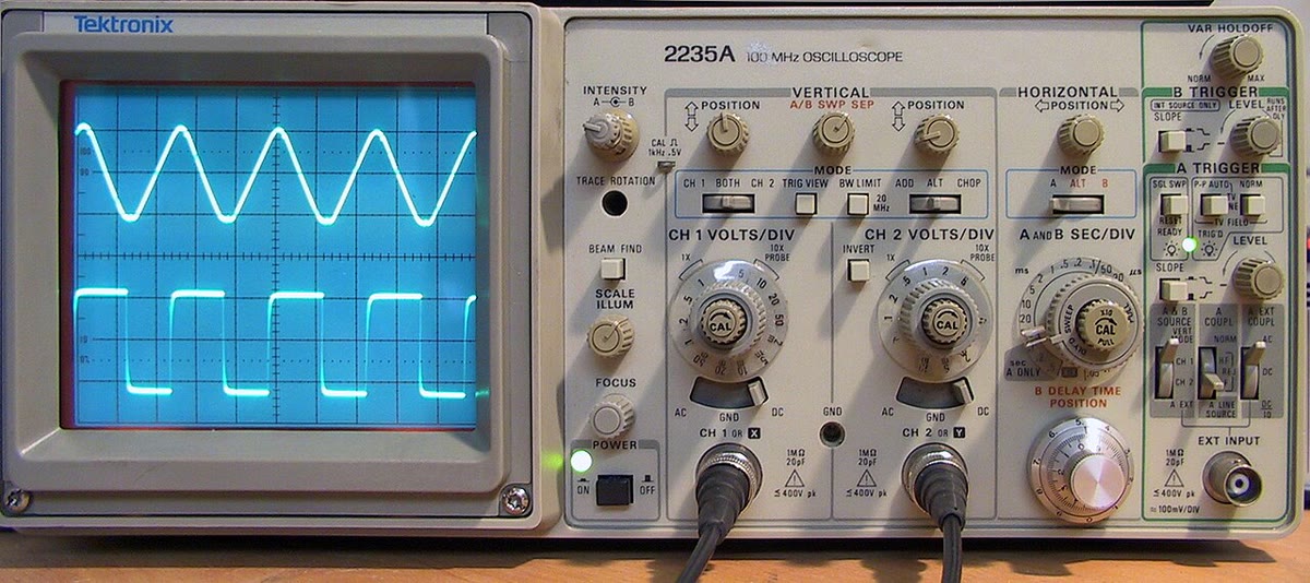
An oscilloscope showing a sinusoid and a square wave: the sinusoid is the signal this chapter lives on, the square wave the one the next chapter decomposes into sinusoids.

8.1 The sinusoidal steady state

Proposition 8.1 (Forced sinusoidal regime)

In a linear circuit driven by a sinusoidal source of angular frequency $\omega$ , every current and voltage is, once the transients have died out, a sinusoid of the same angular frequency $\omega$ , each with its own amplitude and phase: $x(t) = X\cos(\omega t + \varphi)$ .

Proof. The circuit’s equations are linear differential equations with constant coefficients; their general solution is a particular solution plus the solutions of the homogeneous equation, which are the transients of Chapter 7 and decay (every real circuit has some resistance). A sinusoidal particular solution exists because differentiating a sinusoid of frequency $\omega$ gives a sinusoid of the same frequency: the equations can be satisfied term by term — the complex method below constructs it explicitly. ∎

Definition 8.2 (Complex amplitude)

To the sinusoid $x(t) = X\cos(\omega t + \varphi)$ one associates the complex signal $\underline{x}(t) = X\eu^{j(\omega t + \varphi)}$ , so that $x = \Rea(\underline{x})$ , and the complex amplitude

\underline{X} = X\eu^{j\varphi}, \qquad \underline{x}(t) = \underline{X}\,\eu^{j\omega t},

which carries the amplitude $X = \abs{\underline{X}}$ and the phase $\varphi = \arg\underline{X}$ . Here $j$ denotes the imaginary unit, $j^2 = -1$ , the letter $i$ being reserved for currents. Drawn as a vector of length $X$ at angle $\varphi$ , $\underline{X}$ is a phasor (Fresnel vector).

Proposition 8.3 (Rules of the complex method)

Linear operations commute with taking the real part: the complex amplitude of a sum is the sum of the complex amplitudes.
Differentiating with respect to time multiplies the complex amplitude by $j\omega$ ; integrating divides it by $j\omega$ .
Kirchhoff’s laws, being linear, hold for complex amplitudes.

Proof. $\Rea(\underline a + \underline b) = \Rea\underline a + \Rea\underline b$ ; $\dd(\underline X\eu^{j\omega t})/\dd t = j\omega\underline X\eu^{j\omega t}$ , and $\dd x/\dd t = \Rea(\dd\underline x/\dd t)$ since differentiation is real-linear. Sums of currents at a node and of voltages around a loop are linear. ∎

Example 8.4 (Adding two sinusoids)

$3\cos\omega t + 4\sin\omega t$ : the complex amplitudes are $3$ and $4\eu^{-j\pi/2} = -4j$ (since $\sin\omega t = \cos(\omega t - \pi/2)$ ); their sum $3 - 4j$ has modulus $5$ and argument $-0.927\ \mathrm{rad}$ : $5\cos(\omega t - 0.927)$ . No trigonometric identity needed.

8.2 Impedance

Definition 8.5 (Impedance, admittance)

For a linear dipole in the sinusoidal steady state (receiver convention), the impedance is the ratio of complex amplitudes

\underline Z = \frac{\underline U}{\underline I} = Z\eu^{j\varphi} \quad (\text{ohms}),

whose modulus $Z = U/I$ relates the amplitudes and whose argument $\varphi = \varphi_u - \varphi_i$ is the phase lead of the voltage over the current. Its inverse $\underline Y = 1/\underline Z$ is the admittance (siemens). The real part of $\underline Z$ is its resistance, the imaginary part its reactance.

Proposition 8.6 (Impedances of R, L, C)

\underline Z_R = R, \qquad \underline Z_L = jL\omega, \qquad \underline Z_C = \frac{1}{jC\omega} = -\frac{j}{C\omega} .

A resistor keeps voltage and current in phase; in a coil the voltage leads the current by $\pi/2$ ; in a capacitor it lags by $\pi/2$ . At low frequency a coil tends to a wire and a capacitor to an open circuit; at high frequency the reverse.

Proof. $u = Ri$ ; $u = L\,\dd i/\dd t \to \underline U = jL\omega\,\underline I$ ; $i = C\,\dd u/\dd t \to \underline I = jC\omega\,\underline U$ . The arguments of $1$ , $j$ and $-j$ are $0$ , $\pi/2$ , $-\pi/2$ . ∎

Proposition 8.7 (Association; dividers; theorems)

Impedances in series add; admittances in parallel add; the voltage and current dividers, Thévenin’s and Norton’s theorems, superposition and Millman’s theorem of Chapter 6 all hold with complex amplitudes and impedances in place of real voltages, currents and resistances.

Proof. Every proof in Chapter 6 used only Kirchhoff’s laws and the linearity of $u = Ri$ , both of which hold in complex form. ∎

Example 8.8 (The RC divider)

A resistor $R$ and a capacitor $C$ in series across $\underline E$ , the output taken across $C$ : $\underline U_C = \underline E\,\dfrac{1/jC\omega} {R + 1/jC\omega} = \dfrac{\underline E}{1 + jRC\omega}$ . Amplitude $E/\sqrt{1 + (RC\omega)^2}$ , phase $-\arctan(RC\omega)$ : full transmission at low frequency, $1/\sqrt2$ and $-45^\circ$ at $\omega = 1/RC$ , a fall as $1/\omega$ beyond — a low-pass filter, the object of Chapter 9.

8.3 The series RLC circuit: resonance

Theorem 8.9 (Current resonance)

A resistor $R$ , a coil $L$ and a capacitor $C$ in series across $e(t) = E\cos\omega t$ carry the current of complex amplitude

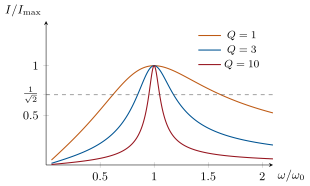
\underline I = \frac{E}{R + j\left(L\omega - \dfrac{1}{C\omega}\right)}, \qquad I = \frac{E}{\sqrt{R^2 + \left(L\omega - \dfrac{1}{C\omega}\right)^2}}, \qquad \varphi_i = -\arctan\frac{L\omega - 1/C\omega}{R} .

The amplitude is maximal, $I_{\max} = E/R$ , with current and voltage in phase, at the resonance $\omega_0 = 1/\sqrt{LC}$ . With $Q = L\omega_0/R = 1/(RC\omega_0)$ and $x = \omega/\omega_0$ ,

\frac{I}{I_{\max}} = \frac{1}{\sqrt{1 + Q^2\left(x - \dfrac1x\right)^2}} ,

and the bandwidth — the interval of $\omega$ over which $I \geq I_{\max}/\sqrt2$ — is

\Delta\omega = \omega_2 - \omega_1 = \frac{\omega_0}{Q} = \frac{R}{L} .

Proof. Series impedances add: $\underline Z = R + jL\omega + 1/jC\omega$ , and $\underline I = \underline E/\underline Z$ . The modulus is largest when the reactance $L\omega - 1/C\omega$ vanishes, i.e. at $\omega_0$ . Factor $L\omega - 1/C\omega = L\omega_0(x - 1/x)$ and divide by $R$ : $L\omega_0/R = Q$ . At the edges of the band, $Q(x - 1/x) = \pm 1$ , i.e. $x^2 \mp x/Q - 1 = 0$ , whose positive roots are $x_{1,2} = \mp\frac{1}{2Q} + \sqrt{1 + \frac{1}{4Q^2}}$ ; their difference is $1/Q$ . ∎

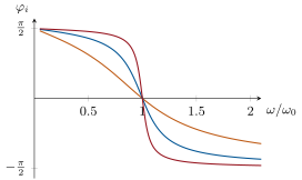
Series RLC: amplitude of the current (left) and its phase relative to the source (right) against / _0, for Q = 1, 3, 10. The peak narrows as Q grows (= _0/Q); below resonance the circuit is capacitive (current leads), above it inductive (current lags). — Series RLC: amplitude of the current (left) and its phase relative to the source (right) against $\omega/\omega_0$ , for $Q = 1, 3, 10$ . The peak narrows as $Q$ grows ( $\Delta\omega = \omega_0/Q$ ); below resonance the circuit is capacitive (current leads), above it inductive (current lags).

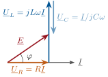
Phasor diagram of the series RLC above resonance: U_R along I, U_L a quarter turn ahead, U_C a quarter turn behind; their sum E leads the current by . At resonance U_L and U_C cancel and E = U_R. — Phasor diagram of the series RLC above resonance: $\underline U_R$ along $\underline I$ , $\underline U_L$ a quarter turn ahead, $\underline U_C$ a quarter turn behind; their sum $\underline E$ leads the current by $\varphi$ . At resonance $\underline U_L$ and $\underline U_C$ cancel and $\underline E = \underline U_R$ .

Proposition 8.10 (Voltage magnification)

At resonance the voltages across the coil and the capacitor have the same amplitude $QE$ and opposite phases: for $Q \gg 1$ the capacitor carries a voltage $Q$ times larger than the source’s. The amplitude $U_C(\omega)$ itself peaks, for $Q > 1/\sqrt2$ , at $\omega_r = \omega_0\sqrt{1 - 1/2Q^2}$ , slightly below $\omega_0$ , with $U_{C,\max} = QE/\sqrt{1 - 1/4Q^2}$ .

Proof. At $\omega_0$ , $\underline U_C = \underline I/jC\omega_0 = -jQE$ and $\underline U_L = jL\omega_0\underline I = jQE$ since $I = E/R$ . In general $U_C = I/C\omega = E/\sqrt{(1 - x^2)^2 + x^2/Q^2}$ (multiply numerator and denominator by $1/C\omega_0$ ); the denominator’s square is $(1 - x^2)^2 + x^2/Q^2$ , a quadratic in $x^2$ minimized at $x^2 = 1 - 1/2Q^2$ when that is positive, with minimum $1/Q^2 - 1/4Q^4$ . ∎

Example 8.11 (Tuning a radio)

A coil $L = 200\,\text{µ}\mathrm{H}$ and a variable capacitor: $C = 127\,\mathrm{pF}$ tunes $f_0 = 1.00\,\mathrm{MHz}$ . With the coil’s wire resistance $R = 12.6\,\Omega$ , $L\omega_0 = 1257\,\Omega$ and $Q = 100$ : bandwidth $\Delta f = f_0/Q = 10\,\mathrm{kHz}$ — the width of an AM channel — and the $10\,\text{µ}\mathrm{V}$ induced by a distant transmitter become $QE = 1\,\mathrm{mV}$ across the capacitor, free of charge. The weekend problem builds this receiver.

Remark 8.12 (Why $Q$ again)

The $Q$ of this chapter is the $Q$ of Chapter 7: the circuit that rings for about $Q$ oscillations when struck is the one that resonates over a band $\omega_0/Q$ wide when driven. Both express one ratio: $2\pi$ times the energy stored over the energy dissipated per period (Exercise 8.12). A sharp resonance and a long ringing are the same property, and so is the slow response: a filter of bandwidth $\Delta\omega$ takes a time of order $1/\Delta\omega$ to settle.

8.4 Power in the sinusoidal regime

Definition 8.13 (RMS value)

The root-mean-square (rms, or effective) value of a periodic signal $x(t)$ is $X_{\mathrm{rms}} = \sqrt{\langle x^2\rangle}$ , the square root of the time average of $x^2$ over a period. For a sinusoid of amplitude $X$ , $X_{\mathrm{rms}} = X/\sqrt2$ . The $230\,\mathrm{V}$ of the mains is an rms value; its amplitude is $325\,\mathrm{V}$ .

Theorem 8.14 (Average power)

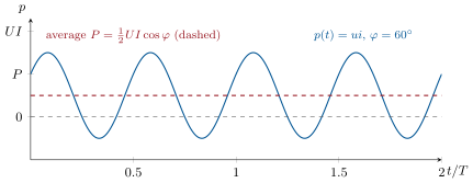
A dipole with $u = U\cos\omega t$ and $i = I\cos(\omega t - \varphi)$ (receiver convention) receives the instantaneous power $p = ui$ , of average

P = \tfrac12\,UI\cos\varphi = U_{\mathrm{rms}}I_{\mathrm{rms}}\cos\varphi = \tfrac12\Rea\!\big(\underline U\,\underline I^{\,*}\big) = \tfrac12\Rea(\underline Z)\,I^2,

where $\cos\varphi$ is the power factor. A resistor receives $\tfrac12 RI^2 = RI_{\mathrm{rms}}^2$ ; an ideal coil or capacitor ( $\varphi = \pm\pi/2$ ) receives no average power — it stores energy during half a period and returns it during the other half.

Proof. $p = UI\cos\omega t\cos(\omega t - \varphi) = \tfrac12 UI[\cos\varphi + \cos(2\omega t - \varphi)]$ ; the second term averages to zero. With $\underline U = U$ and $\underline I = I\eu^{-j\varphi}$ , $\underline U\,\underline I^* = UI\eu^{j\varphi}$ , whose real part is $UI\cos\varphi$ ; and $\underline U = \underline Z\,\underline I$ gives $\underline U\,\underline I^* = \underline Z I^2$ . ∎

Instantaneous power received by a dipole with a 60 phase lag between current and voltage: it pulses at 2, dips below zero (energy returned to the source), and averages to 1/2 UI — here half of what it would be in phase. — Instantaneous power received by a dipole with a $60^\circ$ phase lag between current and voltage: it pulses at $2\omega$ , dips below zero (energy returned to the source), and averages to $\tfrac12 UI\cos\varphi$ — here half of what it would be in phase.

Example 8.15 (Power factor correction)

A workshop motor on $230\,\mathrm{V}$ rms draws $2.0\,\mathrm{kW}$ with $\cos\varphi = 0.70$ (inductive): $I_{\mathrm{rms}} = 2000/(230 \times 0.70) = 12.4\,\mathrm{A}$ , against $8.7\,\mathrm{A}$ if the power factor were $1$ — the extra current heats the utility’s cables for nothing, hence the penalty. A capacitor in parallel supplies the coil’s quarter-period energy swings locally: the reactive power $P\tan\varphi = 2.0\,\mathrm{kvar}$ needs $C = P\tan\varphi/(\omega U_{\mathrm{rms}}^2) \approx 120\,\text{µ}\mathrm{F}$ at $50\,\mathrm{Hz}$ , and the line current drops to $8.7\,\mathrm{A}$ .

8.5 Exercises

Exercise 8.1 ★

Give the complex amplitude of $u = 5\cos(\omega t + \pi/3)$ (V), in polar and Cartesian form. Using complex amplitudes, write $3\cos\omega t + 4\sin\omega t$ as a single cosine.

Solution

Solution of Exercise 8.1.

$\underline U = 5\eu^{j\pi/3} = 2.5 + 4.33j$ (V). $3\cos\omega t + 4\sin\omega t$ : $3 + 4\eu^{-j\pi/2} = 3 - 4j$ , modulus $5$ , argument $-\arctan(4/3) = -0.927\,\mathrm{rad}$ : $5\cos(\omega t - 0.927)$ .

Exercise 8.2 ★

Compute the impedance of $R = 100\,\Omega$ , $L = 0.10\,\mathrm{H}$ and $C = 10\,\text{µ}\mathrm{F}$ at $50\,\mathrm{Hz}$ and at $1.0\,\mathrm{kHz}$ . Give the modulus and phase of the impedance of $R$ and $L$ in series at $50\,\mathrm{Hz}$ .

Solution

Solution of Exercise 8.2.

$R$ : $100\,\Omega$ at both. $L\omega$ : $31.4\,\Omega$ ( $50\,\mathrm{Hz}$ ), $628\,\Omega$ ( $1\,\mathrm{kHz}$ ). $1/C\omega$ : $318\,\Omega$ , $15.9\,\Omega$ . Series $RL$ at $50\,\mathrm{Hz}$ : $\abs{\underline Z} = \sqrt{100^2 + 31.4^2} = 105\,\Omega$ , phase $\arctan(0.314) = 17^\circ$ .

Exercise 8.3 ★

The mains is $230\,\mathrm{V}$ rms: what is its amplitude? A $2.0\,\mathrm{kW}$ heater: rms and peak current. Show that the average power in a resistor is $RI_{\mathrm{rms}}^2$ .

Solution

Solution of Exercise 8.3.

$U = 230\sqrt2 = 325\,\mathrm{V}$ . $I_{\mathrm{rms}} = 2000/230 = 8.7\,\mathrm{A}$ , peak $12.3\,\mathrm{A}$ . $\langle Ri^2\rangle = R\langle i^2\rangle = RI_{\mathrm{rms}}^2$ by definition of the rms value.

Exercise 8.4 ★

Series RLC: $L = 10\,\mathrm{mH}$ , $C = 100\,\mathrm{nF}$ , $R = 100\,\Omega$ , $E = 1.0\,\mathrm{V}$ . Give $f_0$ , $Q$ , the bandwidth in hertz and the current amplitude at resonance.

Solution

Solution of Exercise 8.4.

$f_0 = 1/(2\pi\sqrt{LC}) = 5.03\,\mathrm{kHz}$ ; $Q = \sqrt{L/C}/R = 3.16$ ; $\Delta f = f_0/Q = 1.6\,\mathrm{kHz}$ ; $I_{\max} = E/R = 10\,\mathrm{mA}$ .

Exercise 8.5 ★★

RC divider, output across $C$ : $R = 1.0\,\mathrm{k}\Omega$ , $C = 159\,\mathrm{nF}$ . At what frequency is the output $1/\sqrt2$ of the input? Give the output amplitude ratio and phase at $1.0\,\mathrm{kHz}$ and at $10\,\mathrm{kHz}$ .

Solution

Solution of Exercise 8.5.

$1/\sqrt2$ at $\omega = 1/RC$ : $f_c = 1/(2\pi RC) = 1.0\,\mathrm{kHz}$ . At $1.0\,\mathrm{kHz}$ : ratio $0.71$ , phase $-45^\circ$ . At $10\,\mathrm{kHz}$ : $RC\omega = 10$ , ratio $1/\sqrt{101} = 0.10$ , phase $-84^\circ$ .

Exercise 8.6 ★★

At some frequency a series RLC has $R = 100\,\Omega$ , $L\omega = 250\,\Omega$ , $1/C\omega = 100\,\Omega$ , and $E = 1.0\,\mathrm{V}$ . Compute $\underline Z$ , the current amplitude and phase, and the three voltage amplitudes; draw the phasor diagram. Is the circuit above or below resonance?

Solution

Solution of Exercise 8.6.

$\underline Z = 100 + j(250 - 100) = 100 + 150j$ : $Z = 180\,\Omega$ , $\arg = 56^\circ$ . $I = 1.0/180 = 5.6\,\mathrm{mA}$ , lagging the source by $56^\circ$ . $U_R = 0.56\,\mathrm{V}$ , $U_L = 1.39\,\mathrm{V}$ , $U_C = 0.56\,\mathrm{V}$ ; phasors: $U_R$ along $I$ , $U_L$ up, $U_C$ down, resultant $1.0\,\mathrm{V}$ . $L\omega > 1/C\omega$ : above resonance (inductive).

Exercise 8.7 ★★

Radio: $L = 200\,\text{µ}\mathrm{H}$ , $C$ adjustable from $50\,$ to $500\,\mathrm{pF}$ . Find the frequency range, the capacitance for $1.00\,\mathrm{MHz}$ , and, with $Q = 100$ , the bandwidth and the attenuation (amplitude ratio) of a station $9\,\mathrm{kHz}$ away. An antenna emf of $10\,\text{µ}\mathrm{V}$ : voltage across $C$ at resonance?

Solution

Solution of Exercise 8.7.

$f_0 = 1/(2\pi\sqrt{LC})$ : $1.59\,\mathrm{MHz}$ ( $50\,\mathrm{pF}$ ) to $0.50\,\mathrm{MHz}$ ( $500\,\mathrm{pF}$ ). At $1.00\,\mathrm{MHz}$ : $C = 1/(4\pi^2f_0^2L) = 127\,\mathrm{pF}$ . $\Delta f = 10\,\mathrm{kHz}$ . Station at $1.009\,\mathrm{MHz}$ : $x = 1.009$ , $Q(x - 1/x) = 1.8$ , ratio $1/\sqrt{1 + 3.2} = 0.49$ . Capacitor voltage $QE = 1.0\,\mathrm{mV}$ .

Exercise 8.8 ★★

Derive the two half-power frequencies of the series RLC and show that their difference is $\omega_0/Q$ and their product $\omega_0^2$ .

Solution

Solution of Exercise 8.8.

$Q(x - 1/x) = \pm1 \Leftrightarrow x^2 \mp x/Q - 1 = 0$ ; positive roots $x_{1,2} = \mp 1/2Q + \sqrt{1 + 1/4Q^2}$ . Difference $1/Q$ , so $\Delta\omega = \omega_0/Q$ ; product $(1 + 1/4Q^2) - 1/4Q^2 = 1$ , so $\omega_1\omega_2 = \omega_0^2$ (the band is symmetric on a log scale).

Exercise 8.9 ★★

A motor on $230\,\mathrm{V}$ rms, $50\,\mathrm{Hz}$ , absorbs $2.0\,\mathrm{kW}$ with $\cos\varphi = 0.70$ . Compute the rms current, the reactive power, the capacitance in parallel that brings the power factor to $1$ , and the new current. The supply line has $0.50\,\Omega$ : Joule losses before and after.

Solution

Solution of Exercise 8.9.

$I = P/(U\cos\varphi) = 2000/(230 \times 0.70) = 12.4\,\mathrm{A}$ . Reactive power $P\tan\varphi = 2000 \times 1.02 = 2.0\,\mathrm{kvar}$ . $C = 2040/(314 \times 230^2) = 123\,\text{µ}\mathrm{F}$ . New current $2000/230 = 8.7\,\mathrm{A}$ . Losses $0.50 \times 12.4^2 = 77\,\mathrm{W}$ before, $0.50 \times 8.7^2 = 38\,\mathrm{W}$ after.

Exercise 8.10 ★★★

Parallel RLC fed by a current source: write the admittance, show that the voltage is maximal at $\omega_0 = 1/\sqrt{LC}$ and equals $RI$ there, and that the bandwidth is $\Delta\omega = 1/RC$ , i.e. $Q = R\sqrt{C/L}$ . Numbers: $R = 10\,\mathrm{k}\Omega$ , $L = 1.0\,\mathrm{mH}$ , $C = 1.0\,\mathrm{nF}$ .

Solution

Solution of Exercise 8.10.

$\underline Y = 1/R + j(C\omega - 1/L\omega)$ ; $\underline U = \underline I/ \underline Y$ is maximal when the susceptance vanishes, at $\omega_0$ , where $U = RI$ . Half-power: $\abs{C\omega - 1/L\omega} = 1/R$ , i.e. $RC\omega_0(x - 1/x) = \pm1$ : $\Delta\omega = \omega_0/(RC\omega_0) = 1/RC$ and $Q = RC\omega_0 = R\sqrt{C/L}$ . Numbers: $\omega_0 = 1.0 \times 10^{6}\,\mathrm{rad}/\mathrm{s}$ ( $f_0 = 159\,\mathrm{kHz}$ ), $Q = 10^4\sqrt{10^{-6}} = 10$ , $\Delta f = 16\,\mathrm{kHz}$ .

Exercise 8.11 ★★★

Show that the capacitor voltage of a series RLC is $U_C = E/\sqrt{(1 - x^2)^2 + x^2/Q^2}$ , that it peaks at $x_r = \sqrt{1 - 1/2Q^2}$ if $Q > 1/\sqrt2$ , and compute $x_r$ and $U_{C,\max}/E$ for $Q = 3.16$ . What happens for $Q < 1/\sqrt2$ ?

Solution

Solution of Exercise 8.11.

$U_C = I/C\omega = E/[C\omega\sqrt{R^2 + (L\omega - 1/C\omega)^2}]$ ; multiply inside by $C\omega$ : $\sqrt{(RC\omega)^2 + (LC\omega^2 - 1)^2} = \sqrt{x^2/Q^2 + (1 - x^2)^2}$ . With $s = x^2$ : $(1 - s)^2 + s/Q^2$ is minimal at $s = 1 - 1/2Q^2$ (if positive), minimum $1/Q^2 - 1/4Q^4$ : $U_{C,\max} = QE/\sqrt{1 - 1/4Q^2}$ . $Q = 3.16$ : $x_r = 0.975$ , $U_{C,\max} = 3.2E$ . For $Q < 1/\sqrt2$ the minimum is at $s = 0$ : $U_C$ decreases monotonically from $E$ , no peak.

Exercise 8.12 ★★★

At resonance of a series RLC, show that the total stored energy $\tfrac12 Li^2 + \tfrac12 Cu_C^2$ is constant and equal to $\tfrac12 LI^2$ , compute the energy dissipated in $R$ per period, and prove that $2\pi\,(\text{stored})/(\text{dissipated per period}) = Q$ .

Solution

Solution of Exercise 8.12.

At resonance $i = I\cos\omega_0 t$ and $u_C = (I/C\omega_0)\sin\omega_0 t$ , so, using $1/C\omega_0^2 = L$ ,

\tfrac12 Li^2 + \tfrac12 Cu_C^2 = \tfrac12 LI^2\cos^2\omega_0 t + \tfrac12 LI^2\sin^2\omega_0 t = \tfrac12 LI^2 .

Dissipated per period: $\tfrac12 RI^2T$ . Ratio $\times 2\pi$ : $2\pi L/(RT) = L\omega_0/R = Q$ .

Tuning a valve radio: turning the knob changes a capacitor, the capacitor sets the resonance frequency of an LC circuit, and the station whose frequency matches is the one heard — the weekend problem. — Tuning a valve radio: turning the knob changes a capacitor, the capacitor sets the resonance frequency of an $LC$ circuit, and the station whose frequency matches is the one heard — the weekend problem.

8.6 Problem: The resonant radio receiver

Problem 8.1

Weekend problem — a coil, a variable capacitor and an antenna: how a series resonance picks one station out of a hundred, multiplies its faint signal by a hundred, and why it cannot be made arbitrarily selective

The antenna is modeled by an ideal sinusoidal emf $e(t) = E\cos\omega t$ in series with a coil $L = 200\,\text{µ}\mathrm{H}$ , whose wire has resistance $R = 12.6\,\Omega$ , and a variable capacitor $C$ . The receiver reads the voltage across $C$ . Later (Part IV) the antenna’s own resistance $R_a = 50\,\Omega$ is taken into account.

Part I — The resonant current.

Write the complex impedance of the series circuit.
Give the complex amplitude of the current, then its amplitude $I(\omega)$ and its phase $\varphi_i(\omega)$ relative to $e$ .
Show that $I$ is maximal at $\omega_0 = 1/\sqrt{LC}$ ; give $I_{\max}$ and the phase then.
What capacitance tunes $f_0 = 1.000\,\mathrm{MHz}$ ? Compute $L\omega_0$ .
Define $Q = L\omega_0/R$ and compute it.
Show that $I/I_{\max} = 1/\sqrt{1 + Q^2(x - 1/x)^2}$ with $x = \omega/\omega_0$ .
State the sign of $\varphi_i$ below and above resonance and interpret (capacitive or inductive behavior).

Part II — Selectivity.

Write the condition defining the two frequencies at which $I = I_{\max}/\sqrt2$ .
Solve it and show that $\Delta\omega = \omega_2 - \omega_1 = \omega_0/Q$ .
Compute the bandwidth $\Delta f$ of this receiver.
A second station broadcasts at $1.010\,\mathrm{MHz}$ , a third at $1.020\,\mathrm{MHz}$ : compute the amplitude ratio $I/I_{\max}$ for each, and the corresponding power ratio in decibels.
AM stations are spaced $9\,$ to $10\,\mathrm{kHz}$ apart. Is the receiver selective enough? What would improve it?
The capacitor can be set between $50\,$ and $500\,\mathrm{pF}$ : what frequency band does the receiver cover?

Part III — Voltage magnification.

Express the complex amplitude of the capacitor voltage and show that at resonance its amplitude is $QE$ .
The antenna emf is $E = 10\,\text{µ}\mathrm{V}$ : compute $I_{\max}$ and the capacitor voltage at resonance. Comment.
Show that the coil voltage has the same amplitude and is in phase opposition with the capacitor voltage at resonance: what does the source “see”?
Compute the energy stored in the circuit at resonance and the energy dissipated per period; check that their ratio times $2\pi$ is $Q$ .
From Chapter 7, what is the time constant $\tau = 2Q/\omega_0$ of this circuit? Why does a very high $Q$ eventually distort speech and music (bandwidth of audio: about $5\,\mathrm{kHz}$ for AM)?
If the coil wire resistance doubled (thinner wire), how would $Q$ , the bandwidth and the capacitor voltage change?

Part IV — The antenna’s resistance, and power.

With $R_a = 50\,\Omega$ in series, recompute $Q$ , the bandwidth and the capacitor voltage for $E = 10\,\text{µ}\mathrm{V}$ . Conclude.
Compute the average power delivered by the antenna emf at resonance and the fraction dissipated in $R_a$ .
The maximum-power theorem would ask for a load resistance equal to $R_a$ : why is that goal in conflict with selectivity?
Real receivers connect the antenna to a tap on the coil, or through a small coupling capacitor. Explain qualitatively what this achieves.
Using $P = \tfrac12 UI\cos\varphi$ , compute the power factor at the two half-power frequencies and explain the name “half-power”.
Summarize the design: what $Q$ buys, what it costs, and the value chosen for a $1\,\mathrm{MHz}$ receiver with $10\,\mathrm{kHz}$ channels.

Solution

Solution of Problem 8.1.

1. $\underline Z = R + j(L\omega - 1/C\omega)$ .

2. $\underline I = E/\underline Z$ ; $I = E/\sqrt{R^2 + (L\omega - 1/C\omega)^2}$ ; $\varphi_i = -\arctan[(L\omega - 1/C\omega)/R]$ .

3. The reactance vanishes at $\omega_0 = 1/\sqrt{LC}$ : $I_{\max} = E/R$ , $\varphi_i = 0$ .

4. $C = 1/(4\pi^2f_0^2L) = 127\,\mathrm{pF}$ ; $L\omega_0 = 2\times10^{-4} \times 6.28\times10^6 = 1257\,\Omega$ .

5. $Q = 1257/12.6 = 100$ .

6. $L\omega - 1/C\omega = L\omega_0(x - 1/x)$ , divide by $R$ .

7. $x < 1$ : reactance negative, $\varphi_i > 0$ , the current leads (capacitive); $x > 1$ : lags (inductive).

8. $Q(x - 1/x) = \pm1$ .

9. $x^2 \mp x/Q - 1 = 0$ , $x_{1,2} = \mp1/2Q + \sqrt{1 + 1/4Q^2}$ , $x_2 - x_1 = 1/Q$ : $\Delta\omega = \omega_0/Q$ .

10. $\Delta f = 10\,\mathrm{kHz}$ .

11. $1.010\,\mathrm{MHz}$ : $Q(x - 1/x) = 100 \times 0.0199 = 2.0$ , ratio $1/\sqrt{5.0} = 0.45$ , power $0.20$ : $-7\,\mathrm{dB}$ . $1.020\,\mathrm{MHz}$ : $3.96$ , ratio $0.25$ , power $0.06$ : $-12\,\mathrm{dB}$ .

12. Marginal: the neighbor is only $7\,\mathrm{dB}$ down. A higher $Q$ (lower $R$ ), or several tuned stages in cascade, sharpens the selection.

13. $0.50\,\mathrm{MHz}$ to $1.59\,\mathrm{MHz}$ : the AM band.

14. $\underline U_C = \underline I/jC\omega$ ; at $\omega_0$ , $U_C = I_{\max}/C\omega_0 = E/(RC\omega_0) = QE$ .

15. $I_{\max} = 10^{-5}/12.6 = 0.79\,\text{µ}\mathrm{A}$ ; $U_C = QE = 1.0\,\mathrm{mV}$ : a hundredfold voltage gain with no amplifier.

16. $\underline U_L = jL\omega_0\underline I = jQE$ , $\underline U_C = -jQE$ : equal and opposite, they cancel; the source sees $R$ alone.

17. Stored $\tfrac12 LI_{\max}^2 = 6.2 \times 10^{-17}\,\mathrm{J}$ ; dissipated per period $\tfrac12 RI_{\max}^2T = 3.9 \times 10^{-18}\,\mathrm{J}$ ; $2\pi \times 6.2/0.39 \approx 100 = Q$ .

18. $\tau = 2Q/\omega_0 = 32\,\text{µ}\mathrm{s}$ . The circuit cannot follow changes faster than $\sim\tau$ : a bandwidth $\Delta f$ passes only modulations slower than $\Delta f$ ; with $Q = 1000$ , $\Delta f = 1\,\mathrm{kHz}$ and the treble of the program would be lost.

19. $Q$ halves to $50$ , $\Delta f$ doubles to $20\,\mathrm{kHz}$ , $U_C$ halves to $0.5\,\mathrm{mV}$ .

20. $R_{\text{tot}} = 62.6\,\Omega$ : $Q = 1257/62.6 = 20$ , $\Delta f = 50\,\mathrm{kHz}$ , $U_C = 20 \times 10\,\text{µ}\mathrm{V} = 0.2\,\mathrm{mV}$ : sensitivity and selectivity both collapse.

21. $P = E^2/(2R_{\text{tot}}) = 10^{-10}/125 = 8 \times 10^{-13}\,\mathrm{W}$ ; fraction in $R_a$ : $50/62.6 = 80\%$ .

22. Matching wants a load resistance equal to $R_a$ , i.e. a large total resistance; selectivity wants the smallest possible total resistance ( $Q = L\omega_0/R_{\text{tot}}$ ). One cannot have both with a direct connection.

23. A tap or a small coupling capacitor presents the antenna with only a fraction of the resonant circuit: the antenna’s resistance is “seen” by the circuit much reduced, keeping $Q$ high, while the antenna still delivers power near its optimum.

24. At the half-power frequencies the reactance equals $\pm R$ , so $\varphi = \pm45^\circ$ and $\cos\varphi = 1/\sqrt2$ ; with $I = I_{\max}/\sqrt2$ too, $P = \tfrac12 EI\cos\varphi$ is half its resonant value.

25. $Q$ multiplies the signal by $Q$ and narrows the band to $f_0/Q$ , at the cost of a slower response ( $\tau = 2Q/\omega_0$ ) and a fragile coupling to the antenna; for $10\,\mathrm{kHz}$ channels at $1\,\mathrm{MHz}$ , $Q \approx 100$ is the number — and the antenna must be coupled lightly to keep it.

Terms defined in this chapter

See all 393 terms in the glossary