University Physics — Year 1 · Bachelor Year 1

1Units, Dimensions, and Measurement

In a basement laboratory a pendulum swings, a stopwatch clicks, and a student writes $g = 9.77\,\mathrm{m}/\mathrm{s}^{2}$ . Is that the “right” value? The textbook says $9.81$ . Whether the two numbers agree, whether the experiment was well designed, which of its steps limited it — none of this can be decided from the digits alone. Physics measures, and a measurement without its uncertainty is a rumor. This chapter sets up the common language of every chapter to come: units, dimensions, orders of magnitude, and the honest arithmetic of uncertainties.

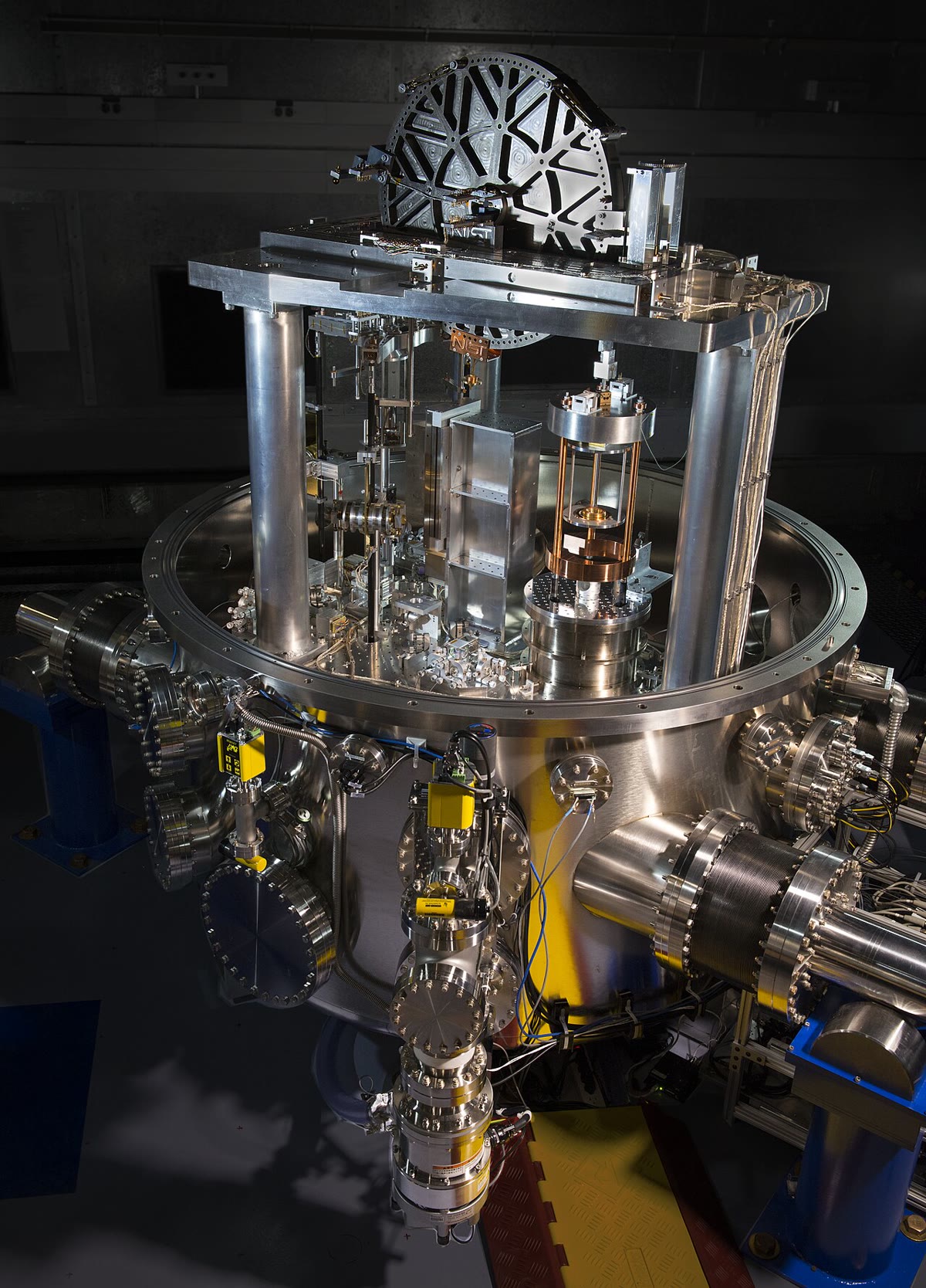
The NIST-4 Kibble balance, one of the instruments that now realize the kilogram from Planck’s constant: a mass is weighed against an electromagnetic force measured in electrical units. Photograph: J. L. Lee, NIST (public domain).

1.1 The International System of Units

Definition 1.1 (Physical quantity and unit)

A physical quantity is a property that can be measured: a length, a duration, a mass, a current. Measuring it means comparing it with a reference quantity of the same kind, the unit: the result is a number times a unit, $\ell = 1.257\,\mathrm{m}$ . The number alone means nothing; the unit alone measures nothing.

Definition 1.2 (Base units of the SI)

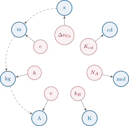
The International System of Units (SI) rests on seven base units: the second ( $\mathrm{s}$ ), the meter ( $\mathrm{m}$ ), the kilogram ( $\mathrm{kg}$ ), the ampere ( $\mathrm{A}$ ), the kelvin ( $\mathrm{K}$ ), the mole ( $\mathrm{mol}$ ) and the candela ( $\mathrm{cd}$ ). Since 2019 each is defined by fixing the numerical value of a constant of nature: the cesium hyperfine frequency $\Delta\nu_{\mathrm{Cs}} = 9\,192\,631\,770\,\mathrm{Hz}$ defines the second; the speed of light $c = 299\,792\,458\,\mathrm{m}/\mathrm{s}$ then defines the meter; the Planck constant $h = 6.626\,070\,15 \times 10^{-34}\,\mathrm{J}\,\mathrm{s}$ defines the kilogram; the elementary charge $e = 1.602\,176\,634 \times 10^{-19}\,\mathrm{C}$ the ampere; the Boltzmann constant $k_B = 1.380\,649 \times 10^{-23}\,\mathrm{J}/\mathrm{K}$ the kelvin; the Avogadro constant $N_A = 6.022\,140\,76 \times 10^{23}\,\mathrm{mol}^{-1}$ the mole; and a fixed luminous efficacy $K_{\mathrm{cd}}$ the candela. Every other unit is a derived unit, a product of powers of base units: $1\,\mathrm{N} = 1\,\mathrm{kg}\,\mathrm{m}/\mathrm{s}^{2}$ , $1\,\mathrm{J} = 1\,\mathrm{N}\,\mathrm{m}$ , $1\,\mathrm{W} = 1\,\mathrm{J}/\mathrm{s}$ , $1\,\mathrm{V} = 1\,\mathrm{W}/\mathrm{A}$ , $1\,\mathrm{Pa} = 1\,\mathrm{N}/\mathrm{m}^{2}$ .

The seven base units (outer ring) and the seven defining constants (inner ring). A fixed constant defines its unit only together with units already defined (dashed): c turns seconds into meters, h needs the meter and the second to define the kilogram, e needs the second to define the ampere. — The seven base units (outer ring) and the seven defining constants (inner ring). A fixed constant defines its unit only together with units already defined (dashed): $c$ turns seconds into meters, $h$ needs the meter and the second to define the kilogram, $e$ needs the second to define the ampere.

Remark 1.3 (Names and symbols)

Units named after people are written lowercase in full (newton, joule, pascal) and capitalized as symbols ( $\mathrm{N}$ , $\mathrm{J}$ , $\mathrm{Pa}$ ); capitalized in full, the word is the person. Prefixes scale by powers of ten, from p ( $10^{-12}$ ) through n, $\mu$ , m, k, M, G to T ( $10^{12}$ ); the kilogram is the one base unit carrying a prefix in its name.

Example 1.4 (Unpacking a derived unit)

The volt: $\mathrm{V} = \mathrm{W}/\mathrm{A} = \mathrm{J}/(\mathrm{A}\,\mathrm{s}) = \mathrm{kg}\,\mathrm{m}^{2}/(\mathrm{A}\,\mathrm{s}^{3})$ . The ohm: $\Omega = \mathrm{V}/\mathrm{A} = \mathrm{kg}\,\mathrm{m}^{2}/(\mathrm{A}^{2}\,\mathrm{s}^{3})$ . The farad: $\mathrm{F} = \mathrm{C}/\mathrm{V} = \mathrm{A}\,\mathrm{s}/\mathrm{V} = \mathrm{A}^{2}\,\mathrm{s}^{4}/(\mathrm{kg}\,\mathrm{m}^{2})$ . Such unpacking is the safest check that a formula has been remembered correctly — the next section makes it systematic.

1.2 Dimensional analysis

Definition 1.5 (Dimension)

The dimension of a quantity $X$ , written $[X]$ , records how $X$ is built from the seven base quantities, independently of the units chosen: length $L$ , mass $M$ , time $T$ , electric current $I$ , temperature $\Theta$ , amount of substance $N$ , luminous intensity $J$ . A speed has dimension $[v] = L\,T^{-1}$ , a force $[F] = M\,L\,T^{-2}$ , an energy $[E] = M\,L^2\,T^{-2}$ . A quantity of dimension $1$ (an angle, a ratio, a refractive index) is dimensionless.

Theorem 1.6 (Principle of dimensional homogeneity)

In a physical law, the two sides of an equality have the same dimension, and every term of a sum has the dimension of the whole. The argument of an exponential, a logarithm, a sine or a cosine is dimensionless.

Proof. The laws of physics do not depend on the units humans choose. Changing the unit of length by a factor $\lambda$ multiplies every quantity of dimension $L^a \cdots$ by $\lambda^{-a}$ : an equality between terms of different dimensions would hold in one system of units and fail in another. For a function such as $\exp$ , the series $1 + x + x^2/2 + \dots$ adds powers of $x$ of different dimensions unless $x$ is dimensionless. ∎

Method 1.7 (Checking a formula)

Write the dimension of every symbol.
Reduce each side (each term) to a product $L^a M^b T^c \cdots$ .
Equal exponents on both sides: the formula may be right. Unequal: it is certainly wrong — a missing factor $g$ , a squared quantity that should be plain, an exponent with dimensions.

A homogeneous formula can still be wrong by a dimensionless factor ( $2$ , $\pi$ , $\tfrac12$ ): dimensions never see those.

Example 1.8 (The period of a pendulum)

A pendulum of length $\ell$ and mass $m$ swings in gravity $g$ . Suppose its period is $\tau = k\,\ell^\alpha m^\beta g^\gamma$ with $k$ dimensionless. Then $T = L^\alpha M^\beta (L T^{-2})^\gamma = L^{\alpha+\gamma} M^\beta T^{-2\gamma}$ , so $\beta = 0$ , $\gamma = -\tfrac12$ , $\alpha = \tfrac12$ :

\tau = k\sqrt{\ell/g} .

Without solving a single equation of motion: the mass drops out, and doubling the length multiplies the period by $\sqrt2$ . Dynamics (Chapter 14) will supply $k = 2\pi$ for small swings.

Proposition 1.9 (Dimensionless groups)

If a quantity $Y$ depends on $n$ quantities $X_1, \dots, X_n$ that involve $r$ independent base dimensions, the relation can be rewritten between $n + 1 - r$ dimensionless combinations of the $X_i$ and $Y$ . When $n + 1 - r = 1$ , the single combination must be a constant, and dimensional analysis gives the law up to a numerical factor.

Proof. Admitted at this level. ∎

Remark 1.10 (Using the proposition)

The general statement (the Vaschy–Buckingham theorem) is a piece of linear algebra on the exponent vectors. What matters here is the recipe: list the relevant quantities, count dimensions, form the dimensionless groups. In Example 1.8, $n = 3$ ( $\ell, m, g$ ), $r = 3$ ( $L, M, T$ ), so a single group $\tau\sqrt{g/\ell}$ exists and must be constant. Drag on a sphere of radius $R$ moving at speed $v$ in a fluid of density $\rho$ and viscosity $\eta$ involves $n = 4$ quantities and $r = 3$ dimensions: two groups, $F/(\rho v^2 R^2)$ and $\rho v R/\eta$ (the Reynolds number), and dimensions alone cannot say how the first depends on the second — experiment must.

1.3 Orders of magnitude

Definition 1.11 (Order of magnitude)

The order of magnitude of a quantity is the power of ten nearest to it: $6.4 \times 10^{6}\,\mathrm{m}$ (the Earth’s radius) has order of magnitude $10^7$ ; $3 \times 10^{3}\,\mathrm{m}$ has order $10^3$ ; $3.2 \times 10^{3}\,\mathrm{m}$ is closer to $10^3$ than to $10^4$ on a logarithmic scale (the boundary is $\sqrt{10} \approx 3.16$ ). Two quantities are “of the same order” when their ratio is below about $3$ .

Method 1.12 (Estimating)

To estimate a quantity nobody has measured for you:

break it into factors you can estimate to within a factor of $2$ or $3$ each;
estimate each factor, keeping one significant figure;
multiply, keeping the power of ten and one digit.

Errors in different factors partly cancel; the result is usually right to within a factor of $3$ to $10$ , which is often all one needs to rule a hypothesis in or out.

Example 1.13 (The mass of the atmosphere)

Atmospheric pressure $P_0 \approx 1 \times 10^{5}\,\mathrm{Pa}$ is the weight of the air column above one square meter, $P_0 = m_{\text{col}}\,g$ , so $m_{\text{col}} \approx 10^5/10 = 1 \times 10^{4}\,\mathrm{kg}$ per square meter. The Earth’s surface is $4\pi R^2 \approx 4 \times 3 \times (6\times10^6)^2 \approx 5 \times 10^{14}\,\mathrm{m}^{2}$ ; the atmosphere weighs about $5 \times 10^{18}\,\mathrm{kg}$ . The accepted value is $5.1 \times 10^{18}\,\mathrm{kg}$ — the estimate needed only $P_0$ and $R$ .

Definition 1.14 (Significant figures)

The significant figures of a written number are its digits from the first non-zero one: $0.0820$ has three, $8.20 \times 10^{-2}$ the same three, $820$ is ambiguous (two or three) unless written $8.2 \times 10^{2}$ or $8.20 \times 10^{2}$ . A result is written with the significant figures its uncertainty allows (Method 1.20 below): not “ $g = 9.7723\,\mathrm{m}/\mathrm{s}^{2}$ ” when the fourth digit is unknown.

1.4 Measurement uncertainty

Definition 1.15 (Measurand, error, uncertainty)

The measurand is the quantity one intends to measure. Repeating a measurement gives scattered values: the measurement is variable. The error of one result is its unknown difference to the true value; the standard uncertainty $u(x)$ of a result $x$ is the standard deviation of the values one could reasonably attribute to the measurand — a quantity one can evaluate. Its sources: the operator (reaction time, parallax), the environment (temperature, vibrations), the instrument (resolution, calibration), the method (a model that is only approximately true).

Proposition 1.16 (Type A evaluation)

From $n$ independent repeated values $x_1, \dots, x_n$ of mean $\bar x = \frac1n \sum x_i$ and experimental standard deviation

s = \sqrt{\frac{1}{n-1}\sum_{i=1}^n (x_i - \bar x)^2},

the best estimate of the measurand is $\bar x$ and its standard uncertainty is

u(\bar x) = \frac{s}{\sqrt n} .

Partial proof. That $s$ estimates the spread of a single measurement is the definition of the experimental standard deviation ( $n - 1$ rather than $n$ because the mean itself was estimated from the data). That the mean of $n$ independent values scatters $\sqrt n$ times less than one value is the addition of variances: the variance of a sum of $n$ independent variables is $n$ times the variance of one, so the variance of the mean is $s^2 n / n^2 = s^2/n$ . The probability course of this year proves both statements. ∎

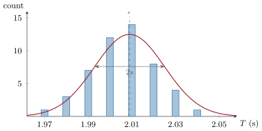
Fifty timings of the same pendulum period, binned by 0.01\, s. Their spread is s 0.016\, s (one timing); the mean of the fifty is known to s/√50 0.002\, s. The bell curve is the Gaussian of the same mean and spread. — Fifty timings of the same pendulum period, binned by $0.01\,\mathrm{s}$ . Their spread is $s \approx 0.016\,\mathrm{s}$ (one timing); the mean of the fifty is known to $s/\sqrt{50} \approx 0.002\,\mathrm{s}$ . The bell curve is the Gaussian of the same mean and spread.

Proposition 1.17 (Type B evaluation)

When a value is read once, its uncertainty is evaluated from what is known of the instrument. If the true value can lie anywhere between $x - a$ and $x + a$ with no preference (a uniform distribution of half-width $a$ ),

u(x) = \frac{a}{\sqrt 3} .

For a scale graduated in steps $\delta$ (half-width $a = \delta/2$ ), $u = \delta/(2\sqrt3) = \delta/\sqrt{12}$ ; the same applies to the last digit of a digital display. A manufacturer’s tolerance quoted as “ $\pm a$ ” is treated the same way unless the data sheet says otherwise.

Proof. The variance of a uniform distribution on $[x - a, x + a]$ is $\frac{1}{2a}\int_{-a}^{a} t^2\,\dd t = \frac{1}{2a}\cdot\frac{2a^3}{3} = \frac{a^2}{3}$ ; its standard deviation is $a/\sqrt3$ . ∎

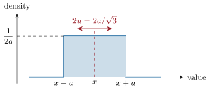
A reading known only to lie within ± a: uniform density 1/(2a), standard deviation a/√3 0.58\,a — smaller than a, because the extremes are no likelier than the center. — A reading known only to lie within $\pm a$ : uniform density $1/(2a)$ , standard deviation $a/\sqrt3 \approx 0.58\,a$ — smaller than $a$ , because the extremes are no likelier than the center.

Theorem 1.18 (Combined uncertainty)

Let $y = f(x_1, \dots, x_n)$ be computed from independent measured values with standard uncertainties $u(x_i)$ . Then

u(y)^2 = \sum_{i=1}^n \left(\frac{\partial f}{\partial x_i}\right)^2 u(x_i)^2 .

In particular:

sum or difference $y = x_1 \pm x_2$ : $u(y)^2 = u(x_1)^2 + u(x_2)^2$ ;
product or quotient $y = x_1 x_2$ or $x_1/x_2$ : $\left(\dfrac{u(y)}{y}\right)^2 = \left(\dfrac{u(x_1)}{x_1}\right)^2 + \left(\dfrac{u(x_2)}{x_2}\right)^2$ ;
power $y = k\,x^\alpha$ : $\dfrac{u(y)}{\abs y} = \abs\alpha\,\dfrac{u(x)}{\abs x}$ .

Proof. For small deviations $\delta x_i$ , the first-order Taylor expansion gives $\delta y = \sum_i (\partial f/\partial x_i)\,\delta x_i$ . The deviations are independent and of zero mean, so the variance of the sum is the sum of the variances, each scaled by the square of its coefficient — the displayed formula. The special cases follow: $\partial(x_1 x_2)/\partial x_1 = x_2$ gives $u(y)^2 = x_2^2 u(x_1)^2 + x_1^2 u(x_2)^2$ , divide by $y^2 = x_1^2 x_2^2$ ; for $y = kx^\alpha$ , $\partial y/\partial x = \alpha y/x$ . ∎

Example 1.19 (The density of a cylinder)

A cylinder: $m = 47.32\,\mathrm{g}$ ( $u = 0.01\,\mathrm{g}$ ), $d = 12.00\,\mathrm{mm}$ ( $u = 0.02\,\mathrm{mm}$ ), $h = 50.2\,\mathrm{mm}$ ( $u = 0.1\,\mathrm{mm}$ ). $\rho = 4m/(\pi d^2 h)$ , so the relative uncertainty squared adds $(0.01/47.32)^2 = 4.5 \times 10^{-8}$ , $(2 \times 0.02/12.00)^2 = 1.1 \times 10^{-5}$ and $(0.1/50.2)^2 = 4.0 \times 10^{-6}$ : the diameter dominates, because it is squared and measured to $0.17\%$ . $u(\rho)/\rho = \sqrt{1.5 \times 10^{-5}} = 0.39\%$ ; $\rho = 8334\,\mathrm{kg}/\mathrm{m}^{3}$ , so $u(\rho) = 33\,\mathrm{kg}/\mathrm{m}^{3}$ : $\rho = (8.33 \pm 0.03)\times10^3\ \mathrm{kg}/\mathrm{m}^{3}$ — brass.

Method 1.20 (Writing a result)

Round the uncertainty to one significant figure (two if the first is $1$ or $2$ ).
Round the value to the same decimal place.
Write value and uncertainty with the unit: $g = (9.77 \pm 0.03)\,\mathrm{m}/\mathrm{s}^{2}$ , or $g = 9.77\,\mathrm{m}/\mathrm{s}^{2}$ , $u(g) = 0.03\,\mathrm{m}/\mathrm{s}^{2}$ .

Keep extra digits during the calculation; round only at the end.

Definition 1.21 (Normalized deviation)

Two results $x_1 \pm u_1$ and $x_2 \pm u_2$ of the same measurand are compared through their normalized deviation

z = \frac{\abs{x_1 - x_2}}{\sqrt{u_1^2 + u_2^2}} .

They are compatible when $z \leq 2$ ; a larger $z$ points to an unaccounted effect — or an underestimated uncertainty. When $x_2$ is a reference value with no quoted uncertainty, take $u_2 = 0$ .

Remark 1.22 (Why 2)

If the two results scatter as Gaussians, their difference has standard deviation $\sqrt{u_1^2 + u_2^2}$ , and a Gaussian exceeds twice its standard deviation in about $5\%$ of cases. “ $z \leq 2$ ” is a convention, not a theorem: it accepts roughly one good measurement in twenty as a false disagreement.

1.5 Fitting a model to data

Proposition 1.23 (Least-squares line)

Given $n$ points $(x_i, y_i)$ expected to obey $y = a x + b$ , the straight line minimizing the sum of squared vertical distances $\sum_i (y_i - a x_i - b)^2$ has

a = \frac{\sum_i (x_i - \bar x)(y_i - \bar y)}{\sum_i (x_i - \bar x)^2}, \qquad b = \bar y - a\,\bar x .

Proof. The sum is a quadratic function of $(a, b)$ ; setting both partial derivatives to zero gives two linear equations: $\sum_i (y_i - ax_i - b) = 0$ , which is $\bar y = a \bar x + b$ , and $\sum_i x_i (y_i - ax_i - b) = 0$ . Substituting $b$ into the second and centering the variables yields $a$ . The minimization itself is carried out in the mathematics course on functions of two variables. ∎

Method 1.24 (Validating a model graphically)

Choose variables that make the expected law a straight line: $\tau^2$ against $\ell$ for the pendulum, $\ln y$ against $\ln x$ for a power law $y = Cx^\alpha$ (slope $\alpha$ ).
Plot the points with their uncertainty bars.
Fit the line; the model is acceptable if the bars straddle the line without a systematic trend of the residuals, and if the intercept is what the model predicts (zero, here).
Read the physics off the slope, with its uncertainty.

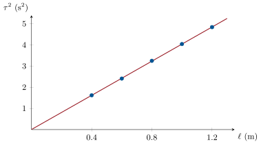
2 against for five pendulum lengths, with uncertainty bars; the least-squares line passes through the origin within uncertainty and its slope 4π2/g gives g. — $\tau^2$ against $\ell$ for five pendulum lengths, with uncertainty bars; the least-squares line passes through the origin within uncertainty and its slope $4\pi^2/g$ gives $g$ .

Example 1.25 (Reading $g$ from a slope)

The five points of the figure have $\bar\ell = 0.800\,\mathrm{m}$ , $\overline{\tau^2} = 3.232\,\mathrm{s}^{2}$ , and the sums $\sum (\ell_i - \bar\ell)(\tau_i^2 - \overline{\tau^2}) = 1.614\,\mathrm{m}\,\mathrm{s}^{2}$ , $\sum (\ell_i - \bar\ell)^2 = 0.400\,\mathrm{m}^{2}$ : slope $a = 4.035\,\mathrm{s}^{2}/\mathrm{m}$ , intercept $b = 0.004\,\mathrm{s}^{2}$ , negligible. With $\tau^2 = (4\pi^2/g)\,\ell$ , $g = 4\pi^2/a = 9.78\,\mathrm{m}/\mathrm{s}^{2}$ .

1.6 Exercises

Exercise 1.1 ★

Express the joule, the watt, the pascal and the coulomb in base units. Deduce that $\mathrm{Pa}\,\mathrm{m}^{3}$ is a unit of energy.

Solution

Solution of Exercise 1.1.

$\mathrm{J} = \mathrm{kg}\,\mathrm{m}^{2}\,\mathrm{s}^{-2}$ ; $\mathrm{W} = \mathrm{kg}\,\mathrm{m}^{2}\,\mathrm{s}^{-3}$ ; $\mathrm{Pa} = \mathrm{kg}\,\mathrm{m}^{-1}\,\mathrm{s}^{-2}$ ; $\mathrm{C} = \mathrm{A}\,\mathrm{s}$ . $\mathrm{Pa}\,\mathrm{m}^{3} = \mathrm{kg}\,\mathrm{m}^{-1}\,\mathrm{s}^{-2}\,\mathrm{m}^{3} = \mathrm{kg}\,\mathrm{m}^{2}\,\mathrm{s}^{-2} = \mathrm{J}$ (the work of pressure forces, $P\,\dd V$ ).

Exercise 1.2 ★

Give the dimensions of a pressure, a power, an electric charge, a voltage, and of the constants $G$ (in $F = Gm_1m_2/r^2$ ), $h$ (in $E = h\nu$ ) and $k_B$ (in $E = k_B T$ ).

Solution

Solution of Exercise 1.2.

Pressure $M L^{-1} T^{-2}$ ; power $M L^2 T^{-3}$ ; charge $I\,T$ ; voltage $=$ power/current $= M L^2 T^{-3} I^{-1}$ . $[G] = [F r^2/m^2] = M L T^{-2} L^2 M^{-2} = L^3 M^{-1} T^{-2}$ ; $[h] = [E/\nu] = M L^2 T^{-2} \cdot T = M L^2 T^{-1}$ ; $[k_B] = [E/T] = M L^2 T^{-2} \Theta^{-1}$ .

Exercise 1.3 ★

Are these formulas homogeneous? $v = \sqrt{2gh}$ ; $E = \tfrac12 m v$ ; $P = \rho g h$ for a pressure; $x = v_0 t + \tfrac12 g t^2$ ; $T = 2\pi\sqrt{g/\ell}$ ; $I = I_0 \eu^{-t/RC}$ .

Solution

Solution of Exercise 1.3.

$\sqrt{2gh}$ : $\sqrt{L T^{-2} \cdot L} = L T^{-1}$ , homogeneous. $\tfrac12 mv$ : $M L T^{-1} \neq M L^2 T^{-2}$ , not an energy. $\rho g h$ : $M L^{-3} \cdot L T^{-2} \cdot L = M L^{-1} T^{-2}$ , a pressure. $v_0 t + \tfrac12 g t^2$ : both terms $L$ , homogeneous. $2\pi\sqrt{g/\ell}$ : $\sqrt{T^{-2}} = T^{-1}$ — a frequency, not a period. $I_0\eu^{-t/RC}$ : $RC$ in $\Omega\,\mathrm{F} = \mathrm{s}$ , argument dimensionless, homogeneous.

Exercise 1.4 ★

A ruler is graduated in millimeters; a digital balance displays $0.01\,\mathrm{g}$ steps; a voltmeter’s data sheet promises “ $\pm 0.5\%$ of the reading”. Give the type B standard uncertainty of a $12.7\,\mathrm{cm}$ length, a $5.43\,\mathrm{g}$ mass and a $4.80\,\mathrm{V}$ reading.

Solution

Solution of Exercise 1.4.

Ruler: $\delta = 1\,\mathrm{mm}$ , $u = 1/\sqrt{12} = 0.29\,\mathrm{mm}$ . Balance: $u = 0.01/\sqrt{12} = 0.003\,\mathrm{g}$ . Voltmeter: $a = 0.005 \times 4.80 = 0.024\,\mathrm{V}$ , $u = 0.024/\sqrt3 = 0.014\,\mathrm{V}$ .

Exercise 1.5 ★★

The speed $v$ of waves on a stretched string depends on its tension $F$ (a force) and its mass per unit length $\mu$ . Find $v$ up to a dimensionless factor. Same question for the speed of sound in a gas of pressure $P$ and density $\rho$ .

Solution

Solution of Exercise 1.5.

$v = k F^\alpha \mu^\beta$ : $L T^{-1} = (M L T^{-2})^\alpha (M L^{-1})^\beta$ , so $\alpha + \beta = 0$ , $\alpha - \beta = 1$ , $-2\alpha = -1$ : $\alpha = \tfrac12$ , $\beta = -\tfrac12$ , $v = k\sqrt{F/\mu}$ (in fact $k = 1$ ). Sound: $P/\rho$ has dimension $M L^{-1} T^{-2} / (M L^{-3}) = L^2 T^{-2}$ , so $v = k\sqrt{P/\rho}$ ( $k = \sqrt\gamma \approx 1.2$ for air).

Exercise 1.6 ★★

Eight timings of the same fall, in milliseconds: $452$ , $447$ , $461$ , $455$ , $449$ , $458$ , $444$ , $454$ . Compute the mean, the experimental standard deviation and the standard uncertainty of the mean; write the result.

Solution

Solution of Exercise 1.6.

Sum $= 3620\,\mathrm{ms}$ , $\bar t = 452.5\,\mathrm{ms}$ . Deviations $-0.5, -5.5, 8.5, 2.5, -3.5, 5.5, -8.5, 1.5$ ; squares sum to $226$ ; $s = \sqrt{226/7} = 5.7\,\mathrm{ms}$ ; $u(\bar t) = 5.7/\sqrt8 = 2.0\,\mathrm{ms}$ . Result: $t = (452.5 \pm 2.0)\,\mathrm{ms}$ .

Exercise 1.7 ★★

A resistance is measured as $R = U/I$ with $U = 4.80\,\mathrm{V}$ , $u(U) = 0.03\,\mathrm{V}$ and $I = 12.4\,\mathrm{mA}$ , $u(I) = 0.2\,\mathrm{mA}$ . Compute $R$ and $u(R)$ ; which measurement should be improved first?

Solution

Solution of Exercise 1.7.

$R = 4.80/0.0124 = 387\,\Omega$ . Relative uncertainties $0.03/4.80 = 0.63\%$ and $0.2/12.4 = 1.6\%$ ; combined $\sqrt{0.63^2 + 1.6^2} = 1.7\%$ , $u(R) = 7\,\Omega$ : $R = (387 \pm 7)\,\Omega$ . The current dominates — improve the ammeter (or its range) first.

Exercise 1.8 ★★

Two groups measure the speed of sound: $(343 \pm 4)\,\mathrm{m}/\mathrm{s}$ and $(336 \pm 3)\,\mathrm{m}/\mathrm{s}$ . Are they compatible? A third group finds $(352 \pm 2)\,\mathrm{m}/\mathrm{s}$ : compatible with the first? with the second?

Solution

Solution of Exercise 1.8.

$z = 7/\sqrt{16 + 9} = 1.4 \leq 2$ : compatible. Third vs first: $z = 9/\sqrt{4 + 16} = 2.0$ : at the limit, barely compatible. Third vs second: $z = 16/\sqrt{4 + 9} = 4.4$ : incompatible — at least one of the two has a systematic error or an underestimated uncertainty.

Exercise 1.9 ★★

The volume of a sphere is computed from its diameter $d = 25.40\,\mathrm{mm}$ measured with a caliper, $u(d) = 0.02\,\mathrm{mm}$ . Compute $V$ , its relative and absolute uncertainty, and write the result.

Solution

Solution of Exercise 1.9.

$V = \pi d^3/6 = \pi \times 25.40^3/6 = 8580\,\mathrm{mm}^{3}$ . $u(V)/V = 3\,u(d)/d = 3 \times 0.02/25.40 = 0.24\%$ , $u(V) = 20\,\mathrm{mm}^{3}$ : $V = (8.58 \pm 0.02)\,\mathrm{cm}^{3}$ .

Exercise 1.10 ★★★

A small sphere of radius $R$ falls slowly in a viscous liquid; the drag depends on $R$ , on the speed $v$ and on the viscosity $\eta$ , of dimension $M L^{-1} T^{-1}$ . Show that $F = k\,\eta R v$ . At high speed the drag depends instead on $R$ , $v$ and the fluid density $\rho$ : find the new law. Estimate, for a raindrop ( $R = 1\,\mathrm{mm}$ , $v = 5\,\mathrm{m}/\mathrm{s}$ , air: $\rho = 1.2\,\mathrm{kg}/\mathrm{m}^{3}$ , $\eta = 1.8 \times 10^{-5}\,\mathrm{Pa}\,\mathrm{s}$ ), which regime applies by comparing the two estimates.

Solution

Solution of Exercise 1.10.

$F = k\eta^a R^b v^c$ : $M$ : $a = 1$ ; $T$ : $-a - c = -2$ , $c = 1$ ; $L$ : $-a + b + c = 1$ , $b = 1$ : $F = k\eta R v$ (Stokes, $k = 6\pi$ ). With $\rho$ instead: $M$ : $a = 1$ ; $T$ : $-c = -2$ , $c = 2$ ; $L$ : $-3 + b + 2 = 1$ , $b = 2$ : $F = k\rho R^2 v^2$ . Raindrop: $\eta R v = 1.8\times10^{-5} \times 10^{-3} \times 5 \approx 1 \times 10^{-7}\,\mathrm{N}$ ; $\rho R^2 v^2 = 1.2 \times 10^{-6} \times 25 = 3 \times 10^{-5}\,\mathrm{N}$ , three hundred times larger: the inertial (high-speed) regime applies — the ratio $\rho v R/\eta \approx 330$ is the Reynolds number.

Exercise 1.11 ★★★

Four measurements of the voltage across a resistor for increasing currents: $(I, U) = (2.0\,\mathrm{mA}, 0.41\,\mathrm{V})$ , $(4.0\,\mathrm{mA}, 0.78\,\mathrm{V})$ , $(6.0\,\mathrm{mA}, 1.22\,\mathrm{V})$ , $(8.0\,\mathrm{mA}, 1.59\,\mathrm{V})$ . Compute the least-squares slope and intercept; deduce $R$ ; is the intercept compatible with zero if each $U$ carries $u = 0.02\,\mathrm{V}$ ?

Solution

Solution of Exercise 1.11.

$\bar I = 5.0\,\mathrm{mA}$ , $\bar U = 1.000\,\mathrm{V}$ ; deviations in $I$ : $-3, -1, 1, 3$ ; in $U$ : $-0.59, -0.22, 0.22, 0.59$ . $\sum (I_i - \bar I)(U_i - \bar U) = 3.98$ , $\sum (I_i - \bar I)^2 = 20$ : $a = 0.199\,\mathrm{V}/\mathrm{mA} = 199\,\Omega$ , $b = 1.000 - 0.199 \times 5 = 0.005\,\mathrm{V}$ . With $u(U) = 0.02\,\mathrm{V}$ per point, an intercept of $0.005\,\mathrm{V}$ is well within uncertainty: compatible with zero, the resistor is ohmic, $R \approx 199\,\Omega$ .

Exercise 1.12 ★★★

From $G = 6.67 \times 10^{-11}\,\mathrm{m}^{3}/(\mathrm{kg}\,\mathrm{s}^{2})$ , $h = 6.63 \times 10^{-34}\,\mathrm{J}\,\mathrm{s}$ and $c = 3.00 \times 10^{8}\,\mathrm{m}/\mathrm{s}$ , build by dimensional analysis a length, a time and a mass (the Planck units). Compute them and compare with the size of a proton ( $1 \times 10^{-15}\,\mathrm{m}$ ) and with a human mass.

Solution

Solution of Exercise 1.12.

$\ell = G^a h^b c^c$ : $M$ : $-a + b = 0$ ; $T$ : $-2a - b - c = 0$ ; $L$ : $3a + 2b + c = 1$ . So $b = a$ , $c = -3a$ , $2a = 1$ : $\ell_P = \sqrt{Gh/c^3} = \sqrt{4.42\times10^{-44}/2.7\times10^{25}} = 4.1 \times 10^{-35}\,\mathrm{m}$ ; $t_P = \ell_P/c = 1.4 \times 10^{-43}\,\mathrm{s}$ ; $m_P = \sqrt{hc/G} = \sqrt{1.99\times10^{-25}/6.67\times10^{-11}} = 5.5 \times 10^{-8}\,\mathrm{kg}$ . The Planck length is twenty orders of magnitude below a proton; the Planck mass, $55\,\text{µ}\mathrm{g}$ , is a speck of dust — huge for a particle, tiny for a person ( $10^9$ times lighter).

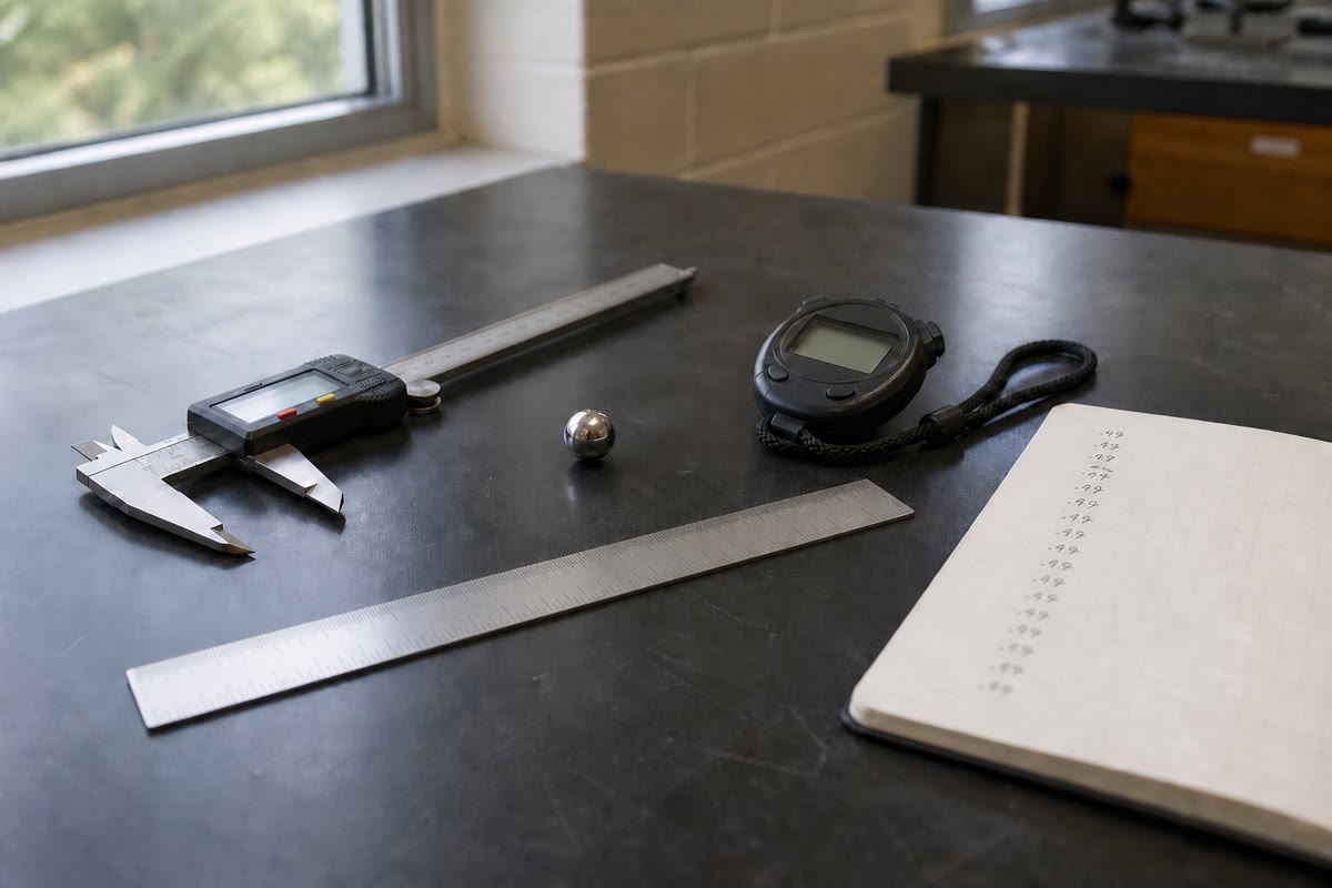
The raw material of the chapter: a caliper, a stopwatch, a ball, a rule, and a column of repeated readings that never quite agree.

1.7 Problem: Measuring $g$ with a pendulum

Problem 1.1

Weekend problem — a string, a bob, a stopwatch and a tape: how well can a kitchen table measure the gravitational field of the Earth, and which of its four numbers is the weak one

A pendulum is a steel ball hung from a fixed point by a light string; small swings have period $\tau = 2\pi\sqrt{\ell/g}$ where $\ell$ is the distance from the suspension point to the ball’s center. The aim is a value of $g$ with a defensible uncertainty.

Part I — The model.

Check the homogeneity of $\tau = 2\pi\sqrt{\ell/g}$ .
The ball has mass $m$ . Argue by dimensions alone that the period cannot depend on $m$ if it depends only on $\ell$ , $g$ and $m$ .
The period also depends, slightly, on the amplitude $\theta_0$ of the swing. Why does dimensional analysis allow this, and what must one do experimentally to make the formula applicable?
Express $g$ as a function of $\ell$ and $\tau$ .

Part II — Measuring the length. The tape measure is graduated in millimeters; the string is $99.0\,\mathrm{cm}$ from suspension to the top of the ball, the ball’s diameter is $2.00\,\mathrm{cm}$ , both read once.

Compute $\ell$ .
Evaluate the type B uncertainty of a single reading on the tape.
Locating the suspension point and the ball’s center adds an estimated $\pm5\,\mathrm{mm}$ of possible error (uniform). Combine with the previous item into $u(\ell)$ , and give the relative uncertainty $u(\ell)/\ell$ .

Part III — Measuring the period. To reduce the effect of reaction time, one times ten periods. Eight such timings, in seconds: $20.12$ , $20.05$ , $20.18$ , $20.09$ , $20.15$ , $20.02$ , $20.11$ , $20.08$ .

Why time ten periods rather than one? Why repeat the timing eight times?
Compute the mean $\overline{t_{10}}$ and the experimental standard deviation $s$ of the eight timings.
Deduce the standard uncertainty of the mean, then the period $\tau$ and its uncertainty $u(\tau)$ .
Compare $u(\tau)/\tau$ with $u(\ell)/\ell$ .

Part IV — The result and its weak point.

Compute $g$ .
Write $u(g)/g$ in terms of $u(\ell)/\ell$ and $u(\tau)/\tau$ , and compute it.
Write the result in the standard form.
Compare with the reference value $9.81\,\mathrm{m}/\mathrm{s}^{2}$ through the normalized deviation. Verdict?
Which of the two measured quantities limits the precision of $g$ ? Propose two concrete improvements and say by how much each would reduce the relative uncertainty.
Suppose that, by a careless alignment, every length was overestimated by $5\,\mathrm{mm}$ . Is this accounted for in the uncertainty budget? What name does this kind of error carry, and how would one detect it?

Part V — Five lengths and a straight line. The experiment is repeated for $\ell = 0.400$ , $0.600$ , $0.800$ , $1.000$ and $1.200\,\mathrm{m}$ , giving $\tau^2 = 1.62$ , $2.41$ , $3.25$ , $4.04$ and $4.84\,\mathrm{s}^{2}$ , each with $u(\tau^2) \approx 1\%$ .

Why plot $\tau^2$ against $\ell$ rather than $\tau$ against $\ell$ ?
Compute $\bar\ell$ and $\overline{\tau^2}$ .
Compute the least-squares slope $a$ and intercept $b$ .
Deduce $g$ from the slope.
Interpret the intercept: what would a clearly non-zero $b$ reveal?
The computer’s fit reports $u(a) = 0.05\,\mathrm{s}^{2}/\mathrm{m}$ . Deduce $u(g)$ and write the result.
Compare the single-length result of Part IV with this one by the normalized deviation.
A student proposes to measure instead one swing of a $10\,\mathrm{m}$ pendulum in a stairwell with the same tape and stopwatch. Estimate the relative uncertainty on $g$ that this would give, and conclude on the best strategy.

Solution

Solution of Problem 1.1.

1. $\sqrt{L/(L T^{-2})} = \sqrt{T^2} = T$ .

2. $\tau = k\ell^\alpha m^\beta g^\gamma$ gives $T = L^{\alpha+\gamma} M^\beta T^{-2\gamma}$ , so $\beta = 0$ : no combination of $\ell$ and $g$ can cancel a mass.

3. $\theta_0$ is dimensionless, so any factor $f(\theta_0)$ is invisible to dimensions. Keep the amplitude small (below about $10^\circ$ ), where $f \approx 1$ to better than $0.2\%$ .

4. $g = 4\pi^2\ell/\tau^2$ .

5. $\ell = 99.0 + 1.00 = 100.0\,\mathrm{cm} = 1.000\,\mathrm{m}$ .

6. $u = 1\,\mathrm{mm}/\sqrt{12} = 0.29\,\mathrm{mm}$ .

7. Alignment: $5/\sqrt3 = 2.9\,\mathrm{mm}$ ; combined $\sqrt{0.29^2 + 2.9^2} = 2.9\,\mathrm{mm}$ — the tape reading is negligible. $u(\ell)/\ell = 0.29\%$ .

8. The reaction-time error (about $0.1\,\mathrm{s}$ ) is the same whether one or ten periods are timed, so its effect on one period is ten times smaller. Repeating reveals the scatter (hence $s$ ) and divides the uncertainty of the mean by $\sqrt8$ .

9. Sum $= 160.80\,\mathrm{s}$ , $\overline{t_{10}} = 20.100\,\mathrm{s}$ . Deviations $0.02, -0.05, 0.08, -0.01, 0.05, -0.08, 0.01, -0.02$ ; squares sum to $188 \times 10^{-4}$ ; $s = \sqrt{188\times10^{-4}/7} = 0.052\,\mathrm{s}$ .

10. $u(\overline{t_{10}}) = 0.052/\sqrt8 = 0.018\,\mathrm{s}$ ; $\tau = 2.0100\,\mathrm{s}$ , $u(\tau) = 0.0018\,\mathrm{s}$ .

11. $u(\tau)/\tau = 0.09\%$ , three times smaller than $u(\ell)/\ell = 0.29\%$ .

12. $g = 4\pi^2 \times 1.000/2.0100^2 = 39.48/4.040 = 9.772\,\mathrm{m}/\mathrm{s}^{2}$ .

13. $g \propto \ell\,\tau^{-2}$ : $\dfrac{u(g)}{g} = \sqrt{\left(\dfrac{u(\ell)}{\ell}\right)^2 + \left(2\dfrac{u(\tau)}{\tau}\right)^2} = \sqrt{0.29^2 + 0.18^2}\,\% = 0.34\%$ .

14. $u(g) = 0.0034 \times 9.772 = 0.033\,\mathrm{m}/\mathrm{s}^{2}$ : $g = (9.77 \pm 0.03)\,\mathrm{m}/\mathrm{s}^{2}$ .

15. $z = \abs{9.772 - 9.81}/0.033 = 1.2 \leq 2$ : compatible.

16. The length ( $0.29\%$ against $0.18\%$ for the period term). Locating both ends to $\pm1\,\mathrm{mm}$ brings $u(\ell)/\ell$ to $0.06\%$ and $u(g)/g$ to $\sqrt{0.06^2 + 0.18^2} = 0.19\%$ ; doubling the length halves $u(\ell)/\ell$ and lengthens $\tau$ , helping both terms. Timing twenty periods instead of ten halves the period term only: $u(g)/g = \sqrt{0.29^2 + 0.09^2} = 0.30\%$ — a small gain while the length is the bottleneck.

17. No: a shift common to every reading is a systematic error (a bias); the budget covers random scatter and declared tolerances, not a consistent offset. It is detected by changing method or instrument, or — Part V — by a non-zero intercept of the $\tau^2$ – $\ell$ line.

18. $\tau^2 = (4\pi^2/g)\,\ell$ is a straight line through the origin: linearity and the zero intercept are both testable by eye and by least squares; $\tau \propto \sqrt\ell$ is not.

19. $\bar\ell = 0.800\,\mathrm{m}$ ; $\overline{\tau^2} = 16.16/5 = 3.232\,\mathrm{s}^{2}$ .

20. Deviations in $\ell$ : $-0.4, -0.2, 0, 0.2, 0.4$ ; in $\tau^2$ : $-1.612, -0.822, 0.018, 0.808, 1.608$ . Cross sum $= 1.614$ , $\sum(\ell_i - \bar\ell)^2 = 0.400$ : $a = 4.035\,\mathrm{s}^{2}/\mathrm{m}$ , $b = 3.232 - 4.035 \times 0.800 = 0.004\,\mathrm{s}^{2}$ .

21. $g = 4\pi^2/a = 39.48/4.035 = 9.78\,\mathrm{m}/\mathrm{s}^{2}$ .

22. $b \approx 0$ , as the model predicts. A clearly non-zero $b$ would betray a systematic offset $\delta$ in every length ( $\tau^2 = a(\ell_{\text{meas}} - \delta)$ gives $b = -a\delta$ ), e.g. a mislocated ball center — or an amplitude effect.

23. $u(g)/g = u(a)/a = 0.05/4.035 = 1.2\%$ , $u(g) = 0.12\,\mathrm{m}/\mathrm{s}^{2}$ : $g = (9.78 \pm 0.12)\,\mathrm{m}/\mathrm{s}^{2}$ .

24. $z = \abs{9.772 - 9.784}/\sqrt{0.033^2 + 0.12^2} = 0.1$ : fully compatible. The single careful measurement is more precise; the line validates the model and guards against a length offset.

25. $\tau = 2\pi\sqrt{10/9.8} = 6.3\,\mathrm{s}$ ; one swing timed with a reaction time of about $0.2\,\mathrm{s}$ gives $u(\tau)/\tau \approx 3\%$ , hence $u(g)/g \approx 6\%$ , while $u(\ell)/\ell$ drops to $0.03\%$ : twenty times worse than Part IV. The length gain is wasted by timing a single period. Best strategy: long pendulum and many periods, repeated — ten swings of the $10\,\mathrm{m}$ pendulum, eight times, gives $u(\tau)/\tau \approx 0.03\%$ and $u(g)/g \approx 0.07\%$ .

Terms defined in this chapter

See all 393 terms in the glossary

1.1 The International System of Units

1.2 Dimensional analysis

1.3 Orders of magnitude

1.4 Measurement uncertainty

1.5 Fitting a model to data

1.6 Exercises

1.7 Problem: Measuring ggg with a pendulum

Terms defined in this chapter

1.7 Problem: Measuring $g$ with a pendulum