University Physics — Year 1 · Bachelor Year 1

26Electrostatics: Field and Gauss’s Law

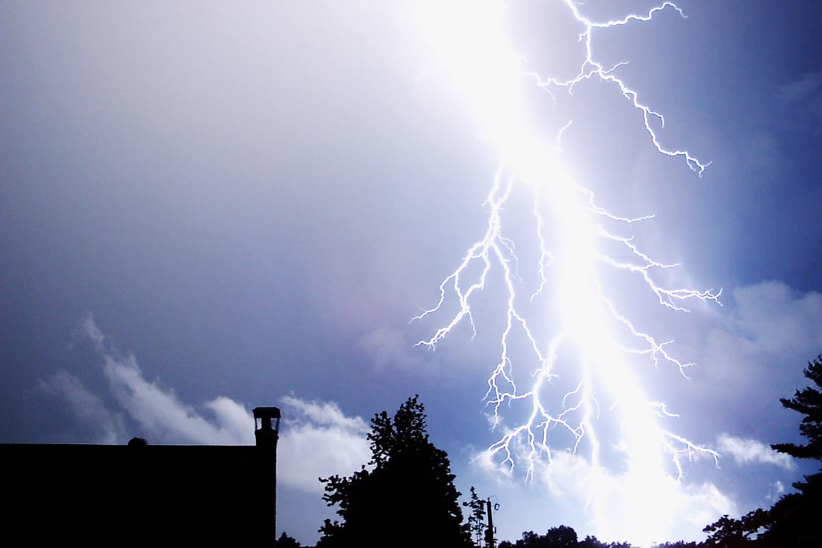
Rub a balloon on a sweater and it sticks to the wall; comb dry hair and the comb bends a thin stream of water. Behind both is the force between electric charges at rest, Coulomb’s law — an inverse-square law like gravity, but $10^{36}$ times stronger between two protons and of both signs, so that matter is neutral to fantastic precision and the residual effects are what we call chemistry, materials and lightning. This chapter builds the concept that makes the law tractable, the electric field, shows how to read a field from its symmetries, and derives the one theorem that computes fields of symmetric distributions in three lines: Gauss’s law. Its gravitational twin comes free at the end.

Cloud-to-ground lightning: tens of coulombs brought down in a few strokes of a hundred kiloamperes — the electric Earth of the weekend problem.

26.1 Charges and Coulomb’s law

Definition 26.1 (Electric charge)

Electric charge $q$ (coulomb, $\mathrm{C}$ ) is a property of matter of either sign; it is conserved (the total charge of an isolated system never changes) and quantized in units of the elementary charge $e = 1.602 \times 10^{-19}\,\mathrm{C}$ (proton $+e$ , electron $-e$ ). A macroscopic distribution is described by a charge density: linear $\lambda$ ( $\mathrm{C}/\mathrm{m}$ ), surface $\sigma$ ( $\mathrm{C}/\mathrm{m}^{2}$ ) or volume $\rho$ ( $\mathrm{C}/\mathrm{m}^{3}$ ), so that a small element carries $\dd q = \lambda\,\dd l$ , $\sigma\,\dd S$ or $\rho\,\dd\tau$ .

Theorem 26.2 (Coulomb’s law)

Two point charges $q_1$ at $M_1$ and $q_2$ at $M_2$ at rest in vacuum exert on each other the forces

\vect F_{1 \to 2} = \frac{q_1q_2}{4\pi\varepsilon_0\,r^2}\,\vect e_{12} = -\vect F_{2 \to 1}, \qquad r = M_1M_2,\quad \vect e_{12} = \frac{\vect{M_1M_2}}{r},

repulsive for like charges, attractive for unlike ones, with the permittivity of vacuum $\varepsilon_0 = 8.854 \times 10^{-12}\,\mathrm{F}/\mathrm{m}$ , i.e. $1/4\pi\varepsilon_0 = 8.99 \times 10^{9}\,\mathrm{N}\,\mathrm{m}^{2}/\mathrm{C}^{2}$ . Forces from several charges add (superposition).

Proof. Admitted at this level. ∎

Example 26.3 (How strong)

Two protons $1\,\mathrm{fm}$ apart repel with $8.99 \times 10^9 \times (1.6 \times 10^{-19})^2/10^{-30} = 230\,\mathrm{N}$ — the weight of a child, between two particles of $10^{-27}$ kg; their gravitational attraction is $10^{36}$ times smaller. Two grams of electrons at one end of a room and the matching protons at the other would attract with $10^{25}$ N. Matter is neutral because it has no choice: any imbalance is corrected by forces no structure can resist.

26.2 The electric field

Definition 26.4 (Electrostatic field)

A distribution of charges at rest creates at every point $M$ of space an electric field $\vect E(M)$ , defined by the force it exerts on a test charge $q$ placed at $M$ : $\vect F = q\vect E(M)$ ( $\mathrm{V}/\mathrm{m}$ $=$ $\mathrm{N}/\mathrm{C}$ ). A point charge $q_1$ at $O$ creates

\vect E(M) = \frac{q_1}{4\pi\varepsilon_0 r^2}\,\vect e_r , \qquad r = OM ,

radial, outward for $q_1 > 0$ ; a distribution creates the vector sum of the fields of its elements. A field line is a curve tangent at each point to $\vect E$ , oriented along it.

Proposition 26.5 (Reading a field map)

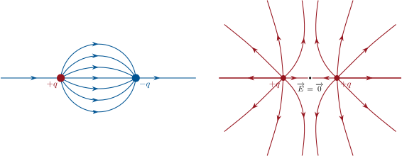
Field lines leave positive charges and end on negative ones (or at infinity); they never cross (the field is single-valued), and they crowd where the field is strong. Where two charges are present, the number of lines drawn from each is proportional to its charge.

Field lines of two opposite charges (left) and of two equal positive charges (right). Lines start on + and end on - or at infinity; on the right they repel each other and the field vanishes at the midpoint, where no line passes. — Field lines of two opposite charges (left) and of two equal positive charges (right). Lines start on $+$ and end on $-$ or at infinity; on the right they repel each other and the field vanishes at the midpoint, where no line passes.

Example 26.6 (Ring and segment by direct summation)

On the axis of a ring of radius $R$ carrying $Q$ uniformly, at distance $z$ from its centre, each element $\dd q$ contributes $\dd q/4\pi\varepsilon_0(R^2 + z^2)$ along the line joining it to $M$ ; the components perpendicular to the axis cancel in pairs and the axial ones add with the factor $z/\sqrt{R^2 + z^2}$ :

E_z = \frac{Qz}{4\pi\varepsilon_0(R^2 + z^2)^{3/2}} ,

zero at the centre, maximal at $z = R/\sqrt2$ , and $Q/4\pi\varepsilon_0z^2$ far away. A uniformly charged disk is a pile of rings (Problem 26.1). Direct summation works whenever the geometry allows the integral; the rest of the chapter is about avoiding it.

26.3 Symmetries and invariances

Proposition 26.7 (Symmetry principle)

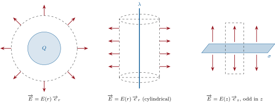
The field has the symmetries of its sources. If a plane $\Pi$ is a plane of symmetry of the charge distribution (the mirror image of the distribution is itself), then at every point of $\Pi$ the field lies in $\Pi$ ; if $\Pi$ is a plane of antisymmetry (the mirror image is the distribution with all charges reversed), the field at points of $\Pi$ is perpendicular to $\Pi$ . If the distribution is invariant under a translation or a rotation, so is the field: its components do not depend on the corresponding coordinate.

Proof. $\vect E$ is a sum of terms $\dd q\,\vect e/4\pi\varepsilon_0r^2$ ; the mirror image of the sum is the sum of the images, and the image of the field of a distribution is the field of the image distribution (a vector built from positions and charges transforms like the positions). On a symmetry plane the field equals its own mirror image, hence lies in the plane; on an antisymmetry plane it equals the opposite of its image, hence is normal to it. Invariance is the same argument with a translation or rotation. ∎

Method 26.8 (Finding the shape of a field before computing it)

For the point $M$ where the field is wanted: (1) list the planes of symmetry of the sources that contain $M$ — the field lies on their intersection; two such planes fix the direction. (2) List the invariances — they tell which coordinates $\vect E$ depends on. Thus a uniformly charged infinite wire gives $\vect E = E(r)\,\vect e_r$ in cylindrical coordinates, a sphere $\vect E = E(r)\,\vect e_r$ in spherical ones, an infinite plane $\vect E = E(z)\,\vect e_z$ with $E(-z) = -E(z)$ . Only then compute.

The three symmetric distributions of the chapter and the Gaussian surfaces (dashed) adapted to them: a concentric sphere, a coaxial cylinder, a pillbox straddling the plane. On each, the field is either normal and uniform in magnitude or tangent.

26.4 Flux and Gauss’s law

Definition 26.9 (Flux of the field)

Cut a surface $S$ into small elements of area $\dd S$ , each with a unit normal $\vect n$ (for a closed surface, the outward normal). The flux of $\vect E$ through $S$ is the sum

\Phi = \sum \vect E\cdot\vect n\,\dd S = \sum E_n\,\dd S \qquad (\mathrm{V}\,\mathrm{m}):

the field’s normal component weighted by area — the “number of field lines” crossing $S$ , counted positively when they cross along $\vect n$ .

Theorem 26.10 (Gauss’s law)

The flux of the electrostatic field through any closed surface $S$ equals the total charge enclosed by $S$ divided by $\varepsilon_0$ :

\Phi_{\text{out}} = \frac{Q_{\text{inside}}}{\varepsilon_0} .

Charges outside $S$ contribute nothing to the flux (their lines go in and come out again).

Proof. For a point charge $q$ at the centre of a sphere of radius $r$ : $\vect E$ is radial, of magnitude $q/4\pi\varepsilon_0r^2$ everywhere on the sphere, so $\Phi = E \times 4\pi r^2 = q/\varepsilon_0$ — independent of $r$ , because the field falls as $1/r^2$ exactly as the area grows. That the same holds for any closed surface around $q$ (the flux through a surface element depends only on the solid angle it subtends from $q$ ), that an outside charge gives zero (it subtends every solid angle twice, with opposite signs), and that the fluxes of several charges add, is admitted here; the full proof is in the Year 2 volume. ∎

Method 26.11 (Using Gauss’s law)

(1) From the symmetries, write the form of $\vect E$ (direction and the variable it depends on). (2) Choose a closed Gaussian surface through the point $M$ on which $\vect E$ is everywhere either normal with the same magnitude $E(M)$ , or tangent: the flux is then $E(M)$ times the area of the normal part. (3) Count the charge inside. (4) Solve for $E(M)$ . It works for spheres, infinite cylinders and infinite planes — and for nothing else without further tools.

Proposition 26.12 (The three classic fields)

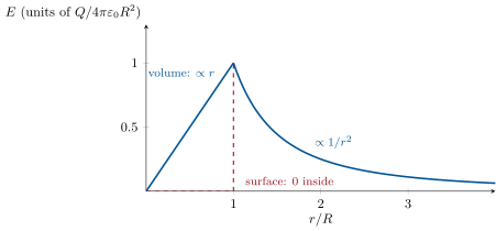
Sphere of radius $R$ , charge $Q$ uniformly spread in its volume: $E(r) = \dfrac{Q}{4\pi\varepsilon_0r^2}$ outside ( $r > R$ ) — as if all the charge sat at the centre — and $E(r) = \dfrac{Qr}{4\pi\varepsilon_0R^3}$ inside, growing linearly from zero; continuous at $r = R$ . If the charge sits on the surface only, the inside field is zero.
Infinite wire of linear charge $\lambda$ : $E(r) = \dfrac{\lambda}{2\pi\varepsilon_0 r}$ , radial.
Infinite plane of surface charge $\sigma$ : $E = \dfrac{\sigma}{2\varepsilon_0}$ on either side, normal to the plane, pointing away from it for $\sigma > 0$ , independent of the distance. Across the plane the normal component jumps by $\sigma/\varepsilon_0$ .

Proof. (1) Sphere of radius $r$ : flux $4\pi r^2E(r)$ ; charge inside $Q$ if $r > R$ , $Q(r/R)^3$ if $r < R$ . (2) Cylinder of radius $r$ , length $h$ : flux through the lateral surface $2\pi rh\,E(r)$ , none through the ends (field tangent); charge $\lambda h$ . (3) Pillbox of cross-section $S$ straddling the plane: flux $2SE$ through the two ends (the field is odd in $z$ , so both count positively), none through the side; charge $\sigma S$ . ∎

The field of a charged sphere against distance from its centre: linear inside and in 1/r2 outside when the charge fills the volume (solid); zero inside and the same outside when it sits on the surface (dashed). Outside, nothing distinguishes the sphere from a point charge at its centre. — The field of a charged sphere against distance from its centre: linear inside and in $1/r^2$ outside when the charge fills the volume (solid); zero inside and the same outside when it sits on the surface (dashed). Outside, nothing distinguishes the sphere from a point charge at its centre.

Example 26.13 (Two planes: the plane capacitor)

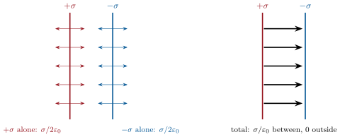
Two parallel planes carrying $+\sigma$ and $-\sigma$ : each creates $\sigma/2\varepsilon_0$ pointing away from it (toward it for the negative one). Between the planes the two fields add to $\sigma/\varepsilon_0$ , directed from $+$ to $-$ ; outside they cancel. With $\sigma = 1\,\text{µ}\mathrm{C}/\mathrm{m}^{2}$ , $E = 10^{-6}/8.85 \times 10^{-12} = 1.1 \times 10^{5}\,\mathrm{V}/\mathrm{m}$ between, zero outside: the field of a charged capacitor is confined to its gap (Chapter 27).

Superposition for two opposite sheets. Left: the uniform fields of each sheet alone (red from the positive one, blue toward the negative one). Right: their sum, / _0 in the gap and zero elsewhere. — Superposition for two opposite sheets. Left: the uniform fields of each sheet alone (red from the positive one, blue toward the negative one). Right: their sum, $\sigma/\varepsilon_0$ in the gap and zero elsewhere.

26.5 The gravitational analogy

Proposition 26.14 (Gauss’s law for gravity)

Newton’s law $\vect F = -Gm_1m_2\,\vect e_{12}/r^2$ has the form of Coulomb’s with $q \to m$ and $1/4\pi\varepsilon_0 \to -G$ . The gravitational field $\vect g$ (force per unit mass) therefore obeys the same symmetry rules and

\Phi_{\text{out}}(\vect g) = -4\pi G\,M_{\text{inside}} .

In particular a spherically symmetric body attracts outside points as if its mass were at its centre, and the field inside a uniform sphere of radius $R$ and mass $M$ is $g(r) = GMr/R^3$ , linear in $r$ .

Proof. Replace $Q/\varepsilon_0$ by $-4\pi GM$ in the proof of Proposition 26.12; the minus sign says the flux enters (gravity attracts). ∎

Example 26.15 (Inside the Earth)

For a uniform Earth, $g$ would fall linearly from $9.8\,\mathrm{m}/\mathrm{s}^{2}$ at the surface to zero at the centre; a stone dropped down a tunnel through the planet would oscillate harmonically with period $2\pi\sqrt{R/g} = 84\,\mathrm{min}$ — the period of a grazing satellite. The real Earth has a dense core, and $g$ actually rises to $10.7\,\mathrm{m}/\mathrm{s}^{2}$ at the core–mantle boundary before falling (Problem 26.1). Newton needed the shell theorem to apply his law to planets; Gauss’s law gives it in a line.

26.6 Exercises

Exercise 26.1 ★

Electric force and gravitational force between two protons $2.0\,\mathrm{fm}$ apart; their ratio. Why then do nuclei hold together?

Solution

Solution of Exercise 26.1.

$F_e = 8.99 \times 10^9 \times (1.6 \times 10^{-19})^2/(2 \times 10^{-15})^2 = 58\,\mathrm{N}$ ; $F_g = 6.67 \times 10^{-11} \times (1.67 \times 10^{-27})^2/(4 \times 10^{-30}) = 4.6 \times 10^{-35}\,\mathrm{N}$ ; ratio $1.2 \times 10^{36}$ . Nuclei hold because the strong interaction, at femtometre range, beats even this repulsion.

Exercise 26.2 ★

Field at $1.0\,\mathrm{m}$ from a $1.0\,\text{µ}\mathrm{C}$ point charge. The Earth’s surface carries a field of $100\,\mathrm{V}/\mathrm{m}$ pointing down: sign and value of the Earth’s charge, treating it as a sphere of radius $6370\,\mathrm{km}$ .

Solution

Solution of Exercise 26.2.

$E = 8.99 \times 10^9 \times 10^{-6}/1 = 9.0\,\mathrm{kV}/\mathrm{m}$ . A downward field is that of a negative charge: $Q = -4\pi\varepsilon_0R^2E = -1.11 \times 10^{-10} \times (6.37 \times 10^6)^2 \times 100 = -4.5 \times 10^{5}\,\mathrm{C}$ .

Exercise 26.3 ★

Two charges $+q$ at $x = \pm a$ on the $x$ axis. Field on the $x$ axis for $|x| > a$ and on the $y$ axis; show that on the $y$ axis $E_y$ is maximal at $y = a/\sqrt2$ . Sketch the lines near the origin.

Solution

Solution of Exercise 26.3.

On the axis, $|x| > a$ : $E_x = \dfrac{q}{4\pi\varepsilon_0}\Bigl[\dfrac{1}{(x - a)^2} + \dfrac{1}{(x + a)^2}\Bigr]$ , outward. On the $y$ axis the $x$ components cancel: $E_y = \dfrac{2qy}{4\pi\varepsilon_0(y^2 + a^2)^{3/2}}$ ; $\dd E_y/\dd y \propto (y^2 + a^2) - 3y^2 = 0$ at $y = a/\sqrt2$ . At the origin the field vanishes; lines leaving each charge toward the other bend away along $\pm y$ — a saddle.

Exercise 26.4 ★

Charges $+2q$ at $x = 0$ and $-q$ at $x = a$ . Where on the $x$ axis does the field vanish? How many field lines leave $+2q$ for each one arriving at $-q$ , and where do the others go?

Solution

Solution of Exercise 26.4.

Between the charges both fields point toward $-q$ : no zero. Left of $+2q$ , $2q/x^2 > q/(x + a)^2$ always. Beyond $-q$ , at distance $d$ from it: $2q/(a + d)^2 = q/d^2$ , $a + d = \sqrt2\,d$ , $d = a/(\sqrt2 - 1) = 2.4a$ . Two lines leave $+2q$ for each one ending on $-q$ ; the other half go to infinity, where the pair looks like a charge $+q$ .

Exercise 26.5 ★★

A disk of radius $R$ carries $\sigma$ uniformly. From the ring result, show that on its axis $E_z = \dfrac{\sigma}{2\varepsilon_0}\Bigl(1 - \dfrac{z}{\sqrt{z^2 + R^2}}\Bigr)$ for $z > 0$ ; check the two limits $z \ll R$ and $z \gg R$ .

Solution

Solution of Exercise 26.5.

Ring of radius $a$ , width $\dd a$ : $\dd q = 2\pi\sigma a\,\dd a$ , $\dd E_z = \dfrac{\sigma z}{2\varepsilon_0}\dfrac{a\,\dd a}{(a^2 + z^2)^{3/2}}$ ; integrate: $\dfrac{\sigma z}{2\varepsilon_0}\Bigl[-\dfrac{1}{\sqrt{a^2 + z^2}}\Bigr]_0^R = \dfrac{\sigma}{2\varepsilon_0} \Bigl(1 - \dfrac{z}{\sqrt{z^2 + R^2}}\Bigr)$ . $z \ll R$ : $\sigma/2\varepsilon_0$ , the infinite plane. $z \gg R$ : $z/\sqrt{z^2 + R^2} \approx 1 - R^2/2z^2$ , so $E_z \approx \sigma R^2/4\varepsilon_0z^2 = Q/4\pi\varepsilon_0z^2$ , the point charge.

Exercise 26.6 ★★

A gold nucleus ( $Z = 79$ , $R = 7.0\,\mathrm{fm}$ ) as a uniformly charged sphere: field at the surface, at $R/2$ , at $1\,\mathrm{pm}$ . Compare with the breakdown field of air, $3 \times 10^{6}\,\mathrm{V}/\mathrm{m}$ .

Solution

Solution of Exercise 26.6.

$Q = 79e = 1.26 \times 10^{-17}\,\mathrm{C}$ ; $E(R) = 8.99 \times 10^9 \times 1.26 \times 10^{-17}/ (7 \times 10^{-15})^2 = 2.3 \times 10^{21}\,\mathrm{V}/\mathrm{m}$ ; at $R/2$ , half: $1.2 \times 10^{21}\,\mathrm{V}/\mathrm{m}$ ; at $1\,\mathrm{pm}$ : $1.14 \times 10^{-7}/10^{-24} = 1.1 \times 10^{17}\,\mathrm{V}/\mathrm{m}$ — $10^{15}$ times the breakdown field of air, at a distance where the electrons live.

Exercise 26.7 ★★

Field of an infinite wire by Gauss’s law. A high-voltage conductor of radius $1.0\,\mathrm{cm}$ : linear charge at which the field at its surface reaches the breakdown value $3 \times 10^{6}\,\mathrm{V}/\mathrm{m}$ (corona onset). Field at $5\,\mathrm{m}$ then.

Solution

Solution of Exercise 26.7.

Cylinder of radius $r$ , length $h$ : $2\pi rh\,E = \lambda h/\varepsilon_0$ , $E = \lambda/2\pi\varepsilon_0r$ . Corona when $\lambda = 2\pi\varepsilon_0 rE = 2\pi \times 8.85 \times 10^{-12} \times 0.01 \times 3 \times 10^6 = 1.7\,\text{µ}\mathrm{C}/\mathrm{m}$ ; at $5\,\mathrm{m}$ , $E = 3 \times 10^6 \times 0.01/5 = 6\,\mathrm{kV}/\mathrm{m}$ .

Exercise 26.8 ★★

Two parallel plates of area $1.0\,\mathrm{m}^{2}$ carry $\pm1.0\,\text{µ}\mathrm{C}$ . Field between them; force on one plate (the field acting on it is that of the other plate only — why?); pressure on the plates.

Solution

Solution of Exercise 26.8.

$E = \sigma/\varepsilon_0 = 10^{-6}/8.85 \times 10^{-12} = 1.1 \times 10^{5}\,\mathrm{V}/\mathrm{m}$ . A plate exerts no net force on itself (its own field’s contributions cancel pairwise); the other plate’s field at its location is $\sigma/2\varepsilon_0$ , so $F = Q\sigma/2\varepsilon_0 = 10^{-6} \times 10^{-6}/(2 \times 8.85 \times 10^{-12}) = 5.6 \times 10^{-2}\,\mathrm{N}$ , attractive; pressure $\sigma^2/2\varepsilon_0 = 0.056\,\mathrm{Pa}$ .

Exercise 26.9 ★★

Coaxial cable: inner conductor of radius $a$ with $+\lambda$ , outer sheath of radius $b$ with $-\lambda$ . Field in the three regions by Gauss’s law. $a = 0.5\,\mathrm{mm}$ , $b = 2.5\,\mathrm{mm}$ , $\lambda = 10\,\mathrm{nC}/\mathrm{m}$ : field at the inner conductor’s surface.

Solution

Solution of Exercise 26.9.

$r < a$ : the inner conductor’s charge sits on its surface, no charge inside, $E = 0$ . $a < r < b$ : $E = \lambda/2\pi\varepsilon_0r$ . $r > b$ : enclosed charge $\lambda - \lambda = 0$ , $E = 0$ — the cable radiates no static field. At $r = a$ : $2 \times 8.99 \times 10^9 \times 10^{-8}/(5 \times 10^{-4}) = 3.6 \times 10^{5}\,\mathrm{V}/\mathrm{m}$ .

Exercise 26.10 ★★★

A thick spherical shell $R_1 < r < R_2$ carries $Q$ uniformly in its volume. Field in the three regions; check continuity at $R_1$ and $R_2$ ; where is it maximal? Sketch $E(r)$ . A positive charge placed in the cavity: what force does it feel?

Solution

Solution of Exercise 26.10.

$\rho = 3Q/4\pi(R_2^3 - R_1^3)$ . $r < R_1$ : $E = 0$ . $R_1 < r < R_2$ : $4\pi r^2E = \rho\,\tfrac43\pi(r^3 - R_1^3)/\varepsilon_0$ , so $E = \dfrac{Q}{4\pi\varepsilon_0r^2}\, \dfrac{r^3 - R_1^3}{R_2^3 - R_1^3}$ . $r > R_2$ : $Q/4\pi\varepsilon_0r^2$ . At $R_1$ both sides give $0$ ; at $R_2$ both give $Q/4\pi\varepsilon_0R_2^2$ . In the shell $E \propto r - R_1^3/r^2$ increases, so the maximum is at $R_2$ , after which it falls as $1/r^2$ . In the cavity the field is zero: a charge there feels no force — wherever it sits.

Exercise 26.11 ★★★

Gravity inside the Earth. Core: radius $3480\,\mathrm{km}$ , density $11\,000\,\mathrm{kg}/\mathrm{m}^{3}$ ; mantle to $6370\,\mathrm{km}$ , density $4500\,\mathrm{kg}/\mathrm{m}^{3}$ . (a) Mass of core, of mantle, total (compare with $5.97 \times 10^{24}\,\mathrm{kg}$ ). (b) $g$ at the surface and at the core–mantle boundary. (c) Show that $g$ rises with depth in the mantle if the mantle’s density is below $\tfrac23$ of the mean density of what lies beneath, and check.

Solution

Solution of Exercise 26.11.

(a) Core $\tfrac43\pi(3.48 \times 10^6)^3 \times 11000 = 1.94 \times 10^{24}\,\mathrm{kg}$ ; mantle $\tfrac43\pi[(6.37 \times 10^6)^3 - (3.48 \times 10^6)^3] \times 4500 = 4.08 \times 10^{24}\,\mathrm{kg}$ ; total $6.0 \times 10^{24}\,\mathrm{kg}$ , within $1\%$ . (b) Surface $GM/R^2 = 9.9\,\mathrm{m}/\mathrm{s}^{2}$ ; boundary $6.67 \times 10^{-11} \times 1.94 \times 10^{24}/(3.48 \times 10^6)^2 = 10.7\,\mathrm{m}/\mathrm{s}^{2}$ . (c) $g = GM(r)/r^2$ with $\dd M = 4\pi r^2\rho_m\,\dd r$ : $\dd g/\dd r = 4\pi G\rho_m - 2GM(r)/r^3 = 4\pi G[\rho_m - \tfrac23\bar\rho(r)]$ , where $\bar\rho(r) = M(r)/\tfrac43\pi r^3$ is the mean density below $r$ . $g$ rises with depth ( $\dd g/\dd r < 0$ ) iff $\rho_m < \tfrac23\bar\rho$ . Just below the surface $\bar\rho = 5500$ , $\tfrac23\bar\rho = 3700 < 4500$ : $g$ first dips slightly; at the core boundary $\bar\rho = 11000$ , $7300 > 4500$ : it rises there, to $10.7$ .

Exercise 26.12 ★★★

Thomson’s atom. Model the hydrogen atom as a uniform positive sphere of charge $+e$ and radius $R = 0.10\,\mathrm{nm}$ with the electron free inside. (a) Force on the electron at distance $r$ from the centre. (b) Show that it oscillates harmonically and compute the frequency and the wavelength of the light it would emit. (c) Compare with the ultraviolet lines of hydrogen ( $122\,\mathrm{nm}$ and shorter) and comment on what the model gets right and wrong (Chapter 30).

Solution

Solution of Exercise 26.12.

(a) Inside, $E = er/4\pi\varepsilon_0R^3$ outward; on the electron $\vect F = -\dfrac{e^2}{4\pi\varepsilon_0R^3}\,\vect r$ : a spring. (b) $\omega = \sqrt{e^2/4\pi\varepsilon_0mR^3} = \sqrt{2.31 \times 10^{-28}/(9.11 \times 10^{-31} \times 10^{-30})} = 1.6 \times 10^{16}\,\mathrm{rad}/\mathrm{s}$ , $f = 2.5 \times 10^{15}\,\mathrm{Hz}$ , $\lambda = c/f = 120\,\mathrm{nm}$ . (c) Startlingly close to the $122\,\mathrm{nm}$ line: the size and strength of the atom are right. But the model gives one frequency, not a series, and the nucleus is not a $0.1\,\mathrm{nm}$ ball but a $10^{-15}$ m point — and a classical orbiting electron would radiate its energy away in nanoseconds. The fix is Chapter 30.

26.7 Problem: The electric Earth

Problem 26.1

Weekend problem — the fair-weather field, the thundercloud, the lightning stroke, and Gauss’s law turned on gravity

Data: $\varepsilon_0 = 8.85 \times 10^{-12}\,\mathrm{F}/\mathrm{m}$ , $1/4\pi\varepsilon_0 = 8.99 \times 10^{9}\,\mathrm{SI}$ , $e = 1.6 \times 10^{-19}\,\mathrm{C}$ , Earth’s radius $R_E = 6.37 \times 10^{6}\,\mathrm{m}$ , surface $5.1 \times 10^{14}\,\mathrm{m}^{2}$ , $G = 6.67 \times 10^{-11}\,\mathrm{SI}$ , $M_E = 5.97 \times 10^{24}\,\mathrm{kg}$ .

Part I — The fair-weather field. In clear weather the field at the ground is $E_0 = 100\,\mathrm{V}/\mathrm{m}$ , pointing down.

Direction of the force on a free electron at the ground; sign of the Earth’s charge.
Treat the Earth as a uniformly charged sphere: from Gauss’s law, its total charge.
Surface charge density of the ground; number of excess electrons per square centimetre.
Force on a dust grain of mass $1\,\text{µ}\mathrm{g}$ carrying $100$ elementary charges; compare with its weight.
Measurements show the field falling to about $5\,\mathrm{V}/\mathrm{m}$ at $10\,\mathrm{km}$ . Apply Gauss’s law to a vertical column of cross-section $1\,\mathrm{m}^{2}$ between the ground and $10\,\mathrm{km}$ : sign and amount of the charge the air holds per square metre.
Mean volume charge density of that air, and the corresponding number of elementary charges per cubic metre. (The air contains about $10^9$ ions of each sign per cubic metre: what fraction of imbalance is this?)
The air has a small conductivity $\gamma = 2 \times 10^{-14}\,\mathrm{S}/\mathrm{m}$ , so a current density $\gamma E_0$ flows down. Total fair-weather current over the globe; time it would take to neutralize the Earth’s charge. Conclude.

Part II — The thundercloud. Model a storm cloud as two horizontal disks of radius $R = 3\,\mathrm{km}$ : $-Q$ at altitude $3\,\mathrm{km}$ , $+Q$ at $9\,\mathrm{km}$ , with $Q = 40\,\mathrm{C}$ .

Field on the axis of a ring of radius $a$ carrying $q$ , at distance $z$ from its centre (symmetry, then summation).
Deduce, by summing over rings, the field on the axis of a disk of radius $R$ and surface charge $\sigma$ : $E_z = \dfrac{\sigma}{2\varepsilon_0}\Bigl(1 - \dfrac{z}{\sqrt{z^2 + R^2}}\Bigr)$ .
Limits $z \ll R$ and $z \gg R$ ; interpret each.
Surface charge of the lower disk; field it creates at the ground directly beneath (direction and value).
Field of the upper disk at the same point; net field at the ground under the storm. The ground is a conductor and its induced charges roughly double the result (admitted): compare with the $10\,\mathrm{kV}/\mathrm{m}$ measured under storms and with the fair-weather value.
Flux of the field through a closed surface enclosing the whole cloud; through one enclosing the lower disk only.
Field midway between the two disks ( $6\,\mathrm{km}$ ), and its direction; compare with the breakdown field of air at that altitude, about $1.5 \times 10^{6}\,\mathrm{V}/\mathrm{m}$ .
If the $40\,\mathrm{C}$ were concentrated in a sphere of radius $500\,\mathrm{m}$ : field at its surface. Why is lightning initiation still an open question?

Part III — The stroke. A return stroke carries $5\,\mathrm{C}$ to the ground in $50\,\text{µ}\mathrm{s}$ through a channel $3\,\mathrm{km}$ long; take the field along the channel as $10^5$ V/m.

Mean current.
Work of the electric force on the charge transferred; power during the stroke; compare with humanity’s average power consumption, about $2 \times 10^{13}\,\mathrm{W}$ .
The channel has a radius of $2\,\mathrm{cm}$ : mass of air in it ( $\rho = 1.2\,\mathrm{kg}/\mathrm{m}^{3}$ ), and the temperature it would reach if all the energy heated it at constant volume ( $c_V = 720\,\mathrm{J}/(\mathrm{kg}\,\mathrm{K})$ ). Actual channel temperatures are near $30\,000\,\mathrm{K}$ : where does the rest go?
Thunder: delay per kilometre, and why the sound of a $3\,\mathrm{km}$ channel rumbles for seconds.
Worldwide about $50$ cloud-to-ground strokes occur every second: current they carry downward; compare with Part I and complete the picture of the “global circuit”.

Part IV — Gauss’s law turned on gravity.

Write Gauss’s law for the gravitational field $\vect g$ and justify the constant by the case of a point mass.
Uniform Earth: $g(r)$ inside; value at $r = R_E/2$ .
Real Earth, core of radius $3480\,\mathrm{km}$ and density $11\,000\,\mathrm{kg}/\mathrm{m}^{3}$ : $g$ at the core–mantle boundary; compare with the surface.
A stone dropped down a frictionless tunnel through a uniform Earth: equation of motion, period of the oscillation, speed at the centre.
Sum up: in each of the four parts, what did Gauss’s law replace, and which four numbers are worth remembering?

Solution

Solution of Problem 26.1.

1. $\vect F = -e\vect E$ : upward. A downward field at the surface is the field of a negative charge: the Earth is negative.

2. Sphere of radius $R_E$ , $E_n = -100$ : $Q = 4\pi\varepsilon_0R_E^2E_n = 1.11 \times 10^{-10} \times 4.06 \times 10^{13} \times (-100) = -4.5 \times 10^{5}\,\mathrm{C}$ .

3. $\sigma = \varepsilon_0E_n = -8.9 \times 10^{-10}\,\mathrm{C}/\mathrm{m}^{2}$ ; $8.9 \times 10^{-10}/1.6 \times 10^{-19} = 5.5 \times 10^9$ electrons per square metre, $5.5 \times 10^5$ per square centimetre.

4. $F = 100e \times 100 = 1.6 \times 10^{-15}\,\mathrm{N}$ ; weight $10^{-9} \times 9.8 = 9.8 \times 10^{-9}\,\mathrm{N}$ : six million times larger.

5. Outward normals: top $E_n = -5$ , bottom $E_n = +100$ , sides zero: $\Phi = 95\,\mathrm{V}\,\mathrm{m}$ , so $Q = 95\varepsilon_0 = +8.4 \times 10^{-10}\,\mathrm{C}$ per square metre — positive space charge, almost cancelling the ground’s $-8.9 \times 10^{-10}$ .

6. $\rho = 8.4 \times 10^{-10}/10^4 = 8.4 \times 10^{-14}\,\mathrm{C}/\mathrm{m}^{3}$ : $5 \times 10^5$ elementary charges per cubic metre; against $10^9$ ions of each sign, an imbalance of $5 \times 10^{-4}$ .

7. $J = \gamma E_0 = 2 \times 10^{-12}\,\mathrm{A}/\mathrm{m}^{2}$ ; $I = J \times 5.1 \times 10^{14} = 1.0\,\mathrm{kA}$ ; $Q/I = 4.5 \times 10^5/1000 = 450\,\mathrm{s}$ . The Earth would be neutral in eight minutes: something recharges it continuously.

8. The axis lies in every plane containing it, all planes of symmetry: $\vect E$ is axial. Each $\dd q$ gives $\dd q/4\pi\varepsilon_0(a^2 + z^2)$ along its own direction, of which the axial part is the fraction $z/\sqrt{a^2 + z^2}$ : $E_z = qz/4\pi\varepsilon_0(a^2 + z^2)^{3/2}$ .

9. $\dd q = 2\pi\sigma a\,\dd a$ : $E_z = \dfrac{\sigma z}{2\varepsilon_0}\displaystyle\int_0^R \dfrac{a\,\dd a}{(a^2 + z^2)^{3/2}} = \dfrac{\sigma}{2\varepsilon_0}\Bigl(1 - \dfrac{z}{\sqrt{z^2 + R^2}}\Bigr)$ .

10. $z \ll R$ : $\sigma/2\varepsilon_0$ , the infinite plane (Gauss’s value); $z \gg R$ : $\sigma R^2/4\varepsilon_0z^2 = Q/4\pi\varepsilon_0z^2$ , the point charge.

11. $\sigma = -40/(\pi \times 9 \times 10^6) = -1.4 \times 10^{-6}\,\mathrm{C}/\mathrm{m}^{2}$ ; $\sigma/2\varepsilon_0 = 8.0 \times 10^{4}\,\mathrm{V}/\mathrm{m}$ ; at $z = 3\,\mathrm{km}$ , $1 - 3/\sqrt{18} = 0.29$ : $E = 2.3 \times 10^{4}\,\mathrm{V}/\mathrm{m}$ , pointing up toward the negative charge.

12. Upper disk, $z = 9\,\mathrm{km}$ : $8.0 \times 10^4 \times (1 - 9/\sqrt{90}) = 4.1 \times 10^{3}\,\mathrm{V}/\mathrm{m}$ downward. Net $1.9 \times 10^{4}\,\mathrm{V}/\mathrm{m}$ upward, about $4 \times 10^4$ with the ground’s induced charges: the right order of the $10\,\mathrm{kV}/\mathrm{m}$ measured (the real charge is more spread out and partly screened); reversed and a hundred times the fair-weather field.

13. Whole cloud: net charge zero, flux zero. Lower disk alone: $-Q/\varepsilon_0 = -40/8.85 \times 10^{-12} = -4.5 \times 10^{12}\,\mathrm{V}\,\mathrm{m}$ .

14. Each disk is $3\,\mathrm{km}$ away and gives $2.3 \times 10^4$ ; the upper ( $+$ ) pushes down, the lower ( $-$ ) pulls down: $4.7 \times 10^{4}\,\mathrm{V}/\mathrm{m}$ downward — thirty times below breakdown.

15. $Q/4\pi\varepsilon_0R^2 = 8.99 \times 10^9 \times 40/(2.5 \times 10^5) = 1.4 \times 10^{6}\,\mathrm{V}/\mathrm{m}$ : only a charge packed into half a kilometre reaches breakdown, and measured in-cloud fields are ten times too weak. Local enhancement at drops and ice, or runaway electrons seeded by cosmic rays, are the candidates — how a flash starts is still debated.

16. $I = 5/(5 \times 10^{-5}) = 1 \times 10^{5}\,\mathrm{A}$ .

17. $W = QEd = 5 \times 10^5 \times 3000 = 1.5 \times 10^{9}\,\mathrm{J}$ ( $420\,\mathrm{kW}\mathrm{h}$ ); $P = 1.5 \times 10^9/5 \times 10^{-5} = 3 \times 10^{13}\,\mathrm{W}$ — one and a half times the power of all humanity, for fifty microseconds.

18. Volume $\pi(0.02)^2 \times 3000 = 3.8\,\mathrm{m}^{3}$ , mass $4.5\,\mathrm{kg}$ ; $\Delta T = 1.5 \times 10^9/(4.5 \times 720) = 4.6 \times 10^{5}\,\mathrm{K}$ if nothing escaped. The channel explodes outward (the shock is the thunder), radiates light and radio waves, ionizes and dissociates the air: heating the final channel to $3 \times 10^4$ K is a small part of the bill.

19. $2.9\,\mathrm{s}$ per kilometre. Sound leaves every point of a $3\,\mathrm{km}$ channel at once, from distances that differ by kilometres: it arrives spread over several seconds — the rumble.

20. $50 \times 5 = 250\,\mathrm{A}$ carried to the ground; with the quieter storm currents (point discharge under clouds, charged rain) the total reaches the kiloampere of Part I: storms are the generators of a global circuit whose return path is the fair-weather air.

21. $\Phi_{\text{out}}(\vect g) = -4\pi GM_{\text{in}}$ : for a point mass $g = -GM/r^2$ on a sphere of area $4\pi r^2$ , flux $-4\pi GM$ , independent of $r$ ; the rest follows as for Coulomb.

22. $g(r) = g_0r/R_E$ ; at $R_E/2$ : $4.9\,\mathrm{m}/\mathrm{s}^{2}$ .

23. $M_{\text{core}} = 1.94 \times 10^{24}\,\mathrm{kg}$ , $g = GM_{\text{core}}/R_c^2 = 10.7\,\mathrm{m}/\mathrm{s}^{2}$ — greater than at the surface: the mantle above is lighter than the average of what is beneath.

24. $m\ddot x = -mg_0x/R_E$ : $\omega = \sqrt{g_0/R_E} = 1.24 \times 10^{-3}\,\mathrm{rad}/\mathrm{s}$ , $T = 2\pi/\omega = 5060\,\mathrm{s} = 84\,\mathrm{min}$ , $v_{\max} = \omega R_E = 7.9\,\mathrm{km}/\mathrm{s}$ — the orbital speed of a grazing satellite, whose period is the same.

25. It replaced the sum over every charge of the Earth (I), over the ions of the air (I), and over every shell of rock (IV) — and in II it fixed the limits of the disk sum. Keep: $-5 \times 10^{5}\,\mathrm{C}$ and $1\,\mathrm{kA}$ for the fair-weather Earth; $40\,\mathrm{C}$ and $10^{4}\,\mathrm{V}/\mathrm{m}$ under a storm; $10^{5}\,\mathrm{A}$ and $10^{9}\,\mathrm{J}$ per stroke; $10.7\,\mathrm{m}/\mathrm{s}^{2}$ at the core boundary.

Terms defined in this chapter

See all 393 terms in the glossary