University Physics — Year 1 · Bachelor Year 1

6DC Circuits: Kirchhoff’s Laws and Theorems

Turn the key on a cold morning: the starter groans, the dashboard lights dim for a second, and the car coughs into life. The battery that delivered a steady $12.6\,\mathrm{V}$ a moment ago is down to eleven while the starter draws its hundred and fifty amperes — and the headlights, wired in parallel, pay for it. Everything in that second is governed by two conservation laws and a handful of theorems about linear circuits, which this chapter states, proves, and applies: Kirchhoff’s laws, the models of sources and resistors, dividers, Thévenin and Norton, and the graphical art of finding an operating point.

6.1 Current, voltage, and the quasi-steady regime

Definition 6.1 (Electric current)

The electric current through a surface (a wire’s cross-section) is the charge crossing it per unit time, counted positively in a chosen orientation:

i = \frac{\dd q}{\dd t} \qquad (\text{amperes: } 1\,\mathrm{A} = 1\,\mathrm{C}/\mathrm{s}).

Reversing the orientation changes the sign of $i$ . In a metal the carriers are electrons, which drift against the conventional current direction, at a fraction of a millimeter per second.

Definition 6.2 (Potential and voltage)

Each point of a circuit has an electric potential $V$ (volts), defined up to a constant fixed by choosing a ground ( $V = 0$ ). The voltage between $A$ and $B$ is the potential difference $u_{AB} = V_A - V_B$ , drawn as an arrow from $B$ to $A$ . The energy a charge $q$ loses in going from $A$ to $B$ is $q\,u_{AB}$ (this connects to the electrostatic potential of Chapter 27).

Definition 6.3 (Quasi-steady regime (ARQS))

A circuit of size $\ell$ driven at frequency $f$ is in the quasi-steady regime when the propagation time $\ell/c$ of electrical signals along it is negligible against the period $1/f$ : $\ell \ll c/f$ . The current is then the same at every point of an unbranched wire at each instant, and the laws below apply at each instant to time-varying currents and voltages (lowercase $i$ , $u$ ) exactly as to steady ones ( $I$ , $U$ ).

Example 6.4 (How quasi is quasi)

At $50\,\mathrm{Hz}$ , $c/f = 6000\,\mathrm{km}$ : a house is in the quasi-steady regime. At $1\,\mathrm{MHz}$ , $300\,\mathrm{m}$ : a radio still is. At $2\,\mathrm{GHz}$ , $15\,\mathrm{cm}$ : a phone’s circuit board is not, and its tracks must be treated as transmission lines — a topic of the Year 2 volume.

Theorem 6.5 (Kirchhoff’s laws)

In the quasi-steady regime:

Node law: at a node where several wires meet, the sum of the currents arriving equals the sum of the currents leaving, $\sum_{\text{in}} i_k = \sum_{\text{out}} i_k$ .
Loop law: around any closed loop, the voltages add up to zero when counted with the sign given by a chosen direction of travel: $\sum_{\text{loop}} \pm u_k = 0$ .

Proof. Charge is conserved and, in the quasi-steady regime, does not pile up at a node: what arrives per second leaves per second. The loop law is the statement that the potential is a function of position: going around a loop and back to the starting point, the sum of the potential drops is $V_A - V_A = 0$ . ∎

Notation 6.6 (Conventions and power)

For a two-terminal component (a dipole), the receiver convention draws the voltage arrow and the current arrow in opposite directions; the generator convention draws them in the same direction. In the receiver convention, the power received by the dipole is

p = u\,i \qquad (\text{watts}),

positive for a resistor that heats, negative for a battery that delivers. In the generator convention $p = ui$ is the power delivered.

The two sign conventions for a dipole: arrows opposed (receiver) or aligned (generator). The physics is the same; only the sign of ui is read differently. — The two sign conventions for a dipole: arrows opposed (receiver) or aligned (generator). The physics is the same; only the sign of $ui$ is read differently.

6.2 Dipoles and their models

Definition 6.7 (Characteristic; resistor; Ohm’s law)

The characteristic of a dipole is the curve $i(u)$ (or $u(i)$ ) it imposes. A resistor has a linear characteristic through the origin, Ohm’s law

u = R\,i \qquad (\text{receiver convention}),

$R$ being its resistance (ohms, $1\,\Omega = 1\,\mathrm{V}/\mathrm{A}$ ) and $G = 1/R$ its conductance (siemens). It receives $p = Ri^2 = u^2/R \geq 0$ , dissipated as heat (Joule effect). A wire of length $\ell$ , cross-section $S$ and resistivity $\rho$ has $R = \rho\ell/S$ .

Definition 6.8 (Ideal and real sources)

An ideal voltage source imposes $u = E$ whatever the current; $E$ is its electromotive force (emf). An ideal current source imposes $i = I_N$ whatever the voltage. A real source (battery, generator, power supply) is modeled, in the generator convention, by

u = E - r\,i \quad (\text{Thévenin model: ideal emf } E \text{ in series with } r)

or, equivalently, by $i = I_N - u/r$ (Norton model: ideal current source $I_N = E/r$ in parallel with $r$ ); $r$ is the internal resistance. $E$ is the open-circuit voltage, $I_N = E/r$ the short-circuit current.

Proposition 6.9 (Power balance of a real source)

A real source $(E, r)$ feeding a resistor $R$ delivers $i = E/(R + r)$ and the power

P_R = \frac{E^2 R}{(R + r)^2},

maximal and equal to $E^2/4r$ when $R = r$ (impedance matching), with efficiency $P_R/(Ei) = R/(R + r)$ , only $50\%$ at the maximum.

Proof. Loop law: $E = ri + Ri$ . $P_R = Ri^2$ ; differentiate $R/(R + r)^2$ : $\big[(R + r)^2 - 2R(R + r)\big]/(R + r)^4 = (r - R)/(R + r)^3$ , zero at $R = r$ , positive before and negative after. The source supplies $Ei = (R + r)i^2$ , of which $ri^2$ heats the source itself. ∎

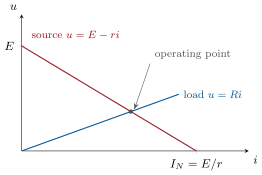
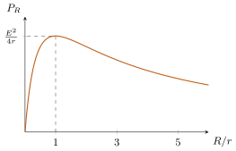
Left: the characteristics of a real source (u = E - ri) and of a resistive load (u = Ri) meet at the operating point. Right: the power delivered to the load peaks at R = r, where half of the source’s power is wasted in its own resistance. — Left: the characteristics of a real source ( $u = E - ri$ ) and of a resistive load ( $u = Ri$ ) meet at the operating point. Right: the power delivered to the load peaks at $R = r$ , where half of the source’s power is wasted in its own resistance.

Example 6.10 (A car battery under load)

Open circuit $12.6\,\mathrm{V}$ ; $11.4\,\mathrm{V}$ while the starter draws $120\,\mathrm{A}$ : $r = 1.2/120 = 10\,\mathrm{m}\Omega$ , $I_N = 1260\,\mathrm{A}$ (hence the welding-grade danger of a dropped spanner). Matched load $R = 10\,\mathrm{m}\Omega$ would take $E^2/4r = 4\,\mathrm{kW}$ for a few seconds — about what a starter motor needs.

Remark 6.11 (Other dipoles)

A diode conducts in one direction only: an idealized model is an open circuit for $u < U_0$ and a fixed voltage $u = U_0$ (about $0.7\,\mathrm{V}$ for silicon, $2\,$ to $3\,\mathrm{V}$ for an LED) when it conducts. A filament lamp is a resistor whose $R$ grows with its temperature, hence with $i$ — a curved characteristic. In steady state a capacitor is an open circuit ( $i = C\,\dd u/\dd t = 0$ ) and an inductor a short circuit ( $u = L\,\dd i/\dd t = 0$ ); their role in transients is Chapter 7.

6.3 Associations and dividers

Proposition 6.12 (Series and parallel resistors)

Resistors in series (same current) add: $R = R_1 + R_2 + \cdots$ . Resistors in parallel (same voltage) add their conductances: $1/R = 1/R_1 + 1/R_2 + \cdots$ ; for two, $R = R_1R_2/(R_1 + R_2)$ , written $R_1 \parallel R_2$ .

Proof. Series: $u = u_1 + u_2 = (R_1 + R_2)i$ (loop law). Parallel: $i = i_1 + i_2 = u/R_1 + u/R_2$ (node law). ∎

Proposition 6.13 (Voltage and current dividers)

Two resistors in series across a voltage $u$ share it in proportion to their resistances:

u_2 = \frac{R_2}{R_1 + R_2}\,u .

Two resistors in parallel fed by a current $i$ share it in inverse proportion:

i_2 = \frac{R_1}{R_1 + R_2}\,i = \frac{G_2}{G_1 + G_2}\,i .

Proof. Series: $i = u/(R_1 + R_2)$ and $u_2 = R_2 i$ . Parallel: $u = (R_1 \parallel R_2)\,i$ and $i_2 = u/R_2$ . ∎

Voltage divider (left): u_2 = R_2 u/(R_1 + R_2). Current divider (right): i_2 = R_1 i/(R_1 + R_2) — the current prefers the smaller resistance. — Voltage divider (left): $u_2 = R_2 u/(R_1 + R_2)$ . Current divider (right): $i_2 = R_1 i/(R_1 + R_2)$ — the current prefers the smaller resistance.

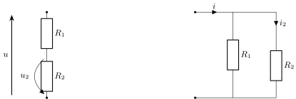
Remark 6.14 (Loading a divider)

The divider formula holds only if nothing draws current from the midpoint. A load $R_L$ connected across $R_2$ replaces $R_2$ by $R_2 \parallel R_L$ and lowers $u_2$ — the “loading effect”, and the reason a voltmeter must have a high resistance and a potentiometer a low one compared with what it feeds (Exercise 6.4).

Method 6.15 (Reducing a network)

To find one current or voltage in a network of resistors and one source:

starting far from the source, replace series and parallel groups by their equivalents until a single resistor faces the source;
compute the source current;
walk back, splitting currents with current dividers and voltages with voltage dividers, down to the wanted branch.

With several sources, or for a branch whose neighbors change, use the theorems of the next section.

6.4 Theorems for linear circuits

Definition 6.16 (Linear dipole, linear circuit)

A dipole is linear if its characteristic is a straight line (resistor, ideal and real sources); a circuit made only of linear dipoles is a linear circuit. Its unknowns obey a system of linear equations (Kirchhoff’s laws plus the characteristics), whose solution is unique.

Theorem 6.17 (Thévenin and Norton)

Seen from two of its terminals $A$ and $B$ , any linear circuit is equivalent to a real source: an emf $E_{\mathrm{Th}}$ in series with a resistance $R_{\mathrm{Th}}$ (Thévenin), or a current source $I_N = E_{\mathrm{Th}}/R_{\mathrm{Th}}$ in parallel with $R_{\mathrm{Th}}$ (Norton), where

$E_{\mathrm{Th}}$ is the open-circuit voltage $u_{AB}$ ;
$I_N$ is the short-circuit current from $A$ to $B$ ;
$R_{\mathrm{Th}}$ is the resistance seen between $A$ and $B$ when every independent source is switched off (ideal voltage sources replaced by wires, ideal current sources by open circuits).

Partial proof. By linearity, the relation between the voltage $u_{AB}$ and the current $i$ drawn at the terminals is affine: $u_{AB} = a - b\,i$ . Setting $i = 0$ identifies $a = E_{\mathrm{Th}}$ ; setting $u_{AB} = 0$ gives $b = E_{\mathrm{Th}}/I_N$ . That $b$ equals the resistance seen with sources killed follows from superposition (below): the part of $u_{AB}$ due to the external current alone is what a passive network of resistance $R_{\mathrm{Th}}$ would produce. That every linear system has an affine input–output relation is the algebra of linear equations. ∎

Theorem 6.18 (Superposition)

In a linear circuit with several independent sources, any current or voltage is the sum of the values it takes when each source acts alone, the others being switched off.

Proof. The equations are linear in the unknowns, with the sources as the right-hand side; the solution is a linear function of that right-hand side, hence the sum of the solutions for each source separately. ∎

Proposition 6.19 (Millman’s theorem)

A node $N$ connected to points of potentials $V_1, \dots, V_n$ through resistances $R_1, \dots, R_n$ (and to nothing else) has the potential

V_N = \frac{\sum_k V_k/R_k}{\sum_k 1/R_k} = \frac{\sum_k G_k V_k}{\sum_k G_k},

the conductance-weighted mean of its neighbors’ potentials.

Proof. Node law at $N$ : $\sum_k (V_k - V_N)/R_k = 0$ ; solve for $V_N$ . ∎

Two sources feeding a common load R_3. Seen from R_3’s terminals, the rest of the circuit is a Thévenin source (E_ Th, R_ Th); Millman’s theorem gives the potential of node N in one line. — Two sources feeding a common load $R_3$ . Seen from $R_3$ ’s terminals, the rest of the circuit is a Thévenin source ( $E_{\mathrm{Th}}$ , $R_{\mathrm{Th}}$ ); Millman’s theorem gives the potential of node $N$ in one line.

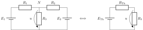
Example 6.20 (Three ways to the same answer)

In the figure, $E_1 = 10\,\mathrm{V}$ , $R_1 = 1.0\,\mathrm{k}\Omega$ , $E_2 = 5.0\,\mathrm{V}$ , $R_2 = 2.0\,\mathrm{k}\Omega$ , $R_3 = 2.0\,\mathrm{k}\Omega$ . Millman: $V_N = (10/1 + 5/2 + 0/2)/(1 + 0.5 + 0.5) = 12.5/2 = 6.25\,\mathrm{V}$ . Superposition: $E_1$ alone sees $R_2 \parallel R_3 = 1\,\mathrm{k}\Omega$ , so $u = 10 \times 1/2 = 5\,\mathrm{V}$ ; $E_2$ alone sees $R_1 \parallel R_3 = 0.667\,\mathrm{k}\Omega$ , $u = 5 \times 0.667/2.667 = 1.25\,\mathrm{V}$ ; total $6.25\,\mathrm{V}$ . Thévenin seen from $R_3$ : $E_{\mathrm{Th}}$ is the open-circuit voltage of the divider $(E_1, R_1, R_2, E_2)$ : $E_2 + (E_1 - E_2)R_2/(R_1 + R_2) = 5 + 5 \times 2/3 = 8.33\,\mathrm{V}$ ; $R_{\mathrm{Th}} = R_1 \parallel R_2 = 0.667\,\mathrm{k}\Omega$ ; then $u = 8.33 \times 2/2.667 = 6.25\,\mathrm{V}$ .

6.5 Operating point; the Wheatstone bridge

Method 6.21 (Graphical operating point)

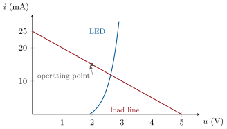
A non-linear dipole (characteristic $i = g(u)$ ) fed by a Thévenin source $(E, R)$ settles where both relations hold: draw the dipole’s characteristic and the source’s load line $u = E - Ri$ on the same axes; their intersection is the operating point. Designing the series resistor of an LED, a Zener regulator or a transistor’s bias is exactly this construction.

An LED (threshold near 2\, V) fed by E = 5\, V through R = 200\,: the load line u = E - Ri crosses the diode’s characteristic at 2.0\, V, 15\, mA. Raising R tilts the line down and dims the LED. — An LED (threshold near $2\,\mathrm{V}$ ) fed by $E = 5\,\mathrm{V}$ through $R = 200\,\Omega$ : the load line $u = E - Ri$ crosses the diode’s characteristic at $2.0\,\mathrm{V}$ , $15\,\mathrm{mA}$ . Raising $R$ tilts the line down and dims the LED.

Proposition 6.22 (Wheatstone bridge)

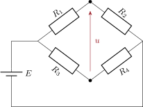
Four resistors $R_1, R_2$ (one branch) and $R_3, R_4$ (the other) across a source $E$ ; the bridge output is the voltage between the two midpoints:

u = E\left(\frac{R_2}{R_1 + R_2} - \frac{R_4}{R_3 + R_4}\right),

zero (the bridge is balanced) iff $R_1R_4 = R_2R_3$ . For a balanced bridge with $R_4$ perturbed to $R_4(1 + \epsilon)$ , $\epsilon \ll 1$ , and $R_3 = R_4$ : $u \approx -E\epsilon/4$ .

Proof. Two voltage dividers; subtract. Balance: $R_2(R_3 + R_4) = R_4(R_1 + R_2)$ , i.e. $R_2R_3 = R_1R_4$ . With $R_3 = R_4 = R$ and $R_1 = R_2$ : $u = E[\tfrac12 - (1 + \epsilon)/(2 + \epsilon)] = E[(2 + \epsilon - 2 - 2\epsilon)/(2(2 + \epsilon))] \approx -E\epsilon/4$ . ∎

The Wheatstone bridge: two dividers side by side. Balanced when R_1R_4 = R_2R_3, it converts a tiny change of one resistance (strain gauge, thermistor) into a voltage around zero, which is far easier to amplify than a small change of a large voltage. — The Wheatstone bridge: two dividers side by side. Balanced when $R_1R_4 = R_2R_3$ , it converts a tiny change of one resistance (strain gauge, thermistor) into a voltage around zero, which is far easier to amplify than a small change of a large voltage.

6.6 Exercises

Exercise 6.1 ★

A phone charges at $1.5\,\mathrm{A}$ for one hour: what charge flows, how many electrons? Estimate whether the quasi-steady regime holds for the house wiring at $50\,\mathrm{Hz}$ , for a $10\,\mathrm{cm}$ circuit at $1\,\mathrm{MHz}$ , and for the same circuit at $1\,\mathrm{GHz}$ .

Solution

Solution of Exercise 6.1.

$q = 1.5 \times 3600 = 5400\,\mathrm{C}$ , $N = 5400/1.6\times10^{-19} = 3.4 \times 10^{22}$ electrons. $c/f$ : $6000\,\mathrm{km}$ at $50\,\mathrm{Hz}$ (house: yes); $300\,\mathrm{m}$ at $1\,\mathrm{MHz}$ ( $10\,\mathrm{cm}$ circuit: yes); $30\,\mathrm{cm}$ at $1\,\mathrm{GHz}$ , comparable to $10\,\mathrm{cm}$ : no.

Exercise 6.2 ★

A $2000\,\mathrm{W}$ heater on $230\,\mathrm{V}$ : current, resistance, energy used in $3.0\,\mathrm{h}$ (in kWh and in joules). Its $5.0\,\mathrm{m}$ copper cord has a cross-section of $1.5\,\mathrm{mm}^{2}$ ( $\rho = 1.7 \times 10^{-8}\,\Omega\,\mathrm{m}$ ): power lost in the cord.

Solution

Solution of Exercise 6.2.

$I = 2000/230 = 8.7\,\mathrm{A}$ ; $R = U^2/P = 26.5\,\Omega$ ; $E = 6.0\,\mathrm{kWh} = 2.2 \times 10^{7}\,\mathrm{J}$ . Cord: one conductor $R = 1.7\times10^{-8} \times 5.0/1.5\times10^{-6} = 57\,\mathrm{m}\Omega$ , two conductors $0.11\,\Omega$ : $P = 0.11 \times 8.7^2 = 8.6\,\mathrm{W}$ .

Exercise 6.3 ★

With $10\,\Omega$ , $20\,\Omega$ and $30\,\Omega$ : compute the resistance of the three in series, in parallel, and of $(10 \parallel 20) + 30$ .

Solution

Solution of Exercise 6.3.

Series $60\,\Omega$ ; parallel $1/(0.1 + 0.05 + 0.033) = 5.5\,\Omega$ ; $10 \parallel 20 = 6.7\,\Omega$ , plus $30$ : $36.7\,\Omega$ .

Exercise 6.4 ★

A $12\,\mathrm{V}$ source feeds $4.7\,\mathrm{k}\Omega$ and $2.2\,\mathrm{k}\Omega$ in series. Compute the voltage across the $2.2\,\mathrm{k}\Omega$ . A device of resistance $2.2\,\mathrm{k}\Omega$ is then connected across it: new voltage? Conclude on the loading effect.

Solution

Solution of Exercise 6.4.

$u_2 = 12 \times 2.2/6.9 = 3.83\,\mathrm{V}$ . Loaded: $2.2 \parallel 2.2 = 1.1\,\mathrm{k}\Omega$ , $u_2 = 12 \times 1.1/5.8 = 2.28\,\mathrm{V}$ : the load pulls the divider down by $40\%$ — a divider only “divides” if it feeds something of much higher resistance.

Exercise 6.5 ★★

A battery reads $12.6\,\mathrm{V}$ open and $11.4\,\mathrm{V}$ while delivering $120\,\mathrm{A}$ . Find its internal resistance and short-circuit current, the power delivered to the starter and the power lost inside, and the efficiency.

Solution

Solution of Exercise 6.5.

$r = (12.6 - 11.4)/120 = 10\,\mathrm{m}\Omega$ ; $I_N = 12.6/0.010 = 1260\,\mathrm{A}$ . To the starter $11.4 \times 120 = 1.37\,\mathrm{kW}$ ; lost $0.010 \times 120^2 = 144\,\mathrm{W}$ ; efficiency $1368/1512 = 90\%$ .

Exercise 6.6 ★★

Find the Thévenin equivalent, seen from the $2.2\,\mathrm{k}\Omega$ resistor’s terminals, of the divider of Exercise 6.4 ( $E = 12\,\mathrm{V}$ , $R_1 = 4.7\,\mathrm{k}\Omega$ , $R_2 = 2.2\,\mathrm{k}\Omega$ ). Use it to recover the loaded voltage of that exercise.

Solution

Solution of Exercise 6.6.

$E_{\mathrm{Th}} = 3.83\,\mathrm{V}$ (open-circuit divider); $R_{\mathrm{Th}} = 4.7 \parallel 2.2 = 1.50\,\mathrm{k}\Omega$ (source shorted). Loaded: $u = 3.83 \times 2.2/(1.50 + 2.2) = 2.28\,\mathrm{V}$ .

Exercise 6.7 ★★

Two batteries, $E_1 = 10\,\mathrm{V}$ ( $r_1 = 1.0\,\Omega$ ) and $E_2 = 5.0\,\mathrm{V}$ ( $r_2 = 2.0\,\Omega$ ), are connected in parallel (same polarity) across a $2.0\,\Omega$ load. Find the load voltage by superposition, then by Millman, and the current in each battery. Is the weaker battery charging or discharging?

Solution

Solution of Exercise 6.7.

Superposition: $E_1$ alone sees $r_2 \parallel R = 1.0\,\Omega$ , $u = 10 \times 1/(1 + 1) = 5.0\,\mathrm{V}$ ; $E_2$ alone sees $r_1 \parallel R = 0.667\,\Omega$ , $u = 5 \times 0.667/2.667 = 1.25\,\mathrm{V}$ ; total $6.25\,\mathrm{V}$ . Millman: $(10/1 + 5/2 + 0/2)/(1 + 0.5 + 0.5) = 6.25\,\mathrm{V}$ . Battery 1: $(10 - 6.25)/1 = 3.75\,\mathrm{A}$ out; battery 2: $(5 - 6.25)/2 = -0.63\,\mathrm{A}$ , i.e. $0.63\,\mathrm{A}$ into it — it is being charged by the stronger one; load $6.25/2 = 3.1\,\mathrm{A}$ .

Exercise 6.8 ★★

A source $E = 9.0\,\mathrm{V}$ , $r = 3.0\,\Omega$ . Compute the power delivered to loads of $1.0\,\Omega$ , $3.0\,\Omega$ , $12\,\Omega$ , and the efficiency in each case. Which load would an engineer choose for a battery-powered device, and why not the matched one?

Solution

Solution of Exercise 6.8.

$i = 9/(R + 3)$ , $P = Ri^2$ , $\eta = R/(R + 3)$ : $1\,\Omega$ : $5.1\,\mathrm{W}$ , $25\%$ ; $3\,\Omega$ : $6.75\,\mathrm{W}$ , $50\%$ ; $12\,\Omega$ : $4.3\,\mathrm{W}$ , $80\%$ . A battery device wants efficiency (battery life), hence $R \gg r$ ; the matched load wastes half the energy as heat in the battery.

Exercise 6.9 ★★

An LED conducts at $2.0\,\mathrm{V}$ and must carry $15\,\mathrm{mA}$ from a $5.0\,\mathrm{V}$ supply. Choose the series resistor, the powers in the resistor and in the LED, and sketch the load line construction. What happens if the supply is $3.3\,\mathrm{V}$ ?

Solution

Solution of Exercise 6.9.

$R = (5.0 - 2.0)/0.015 = 200\,\Omega$ ; $P_R = 3.0 \times 0.015 = 45\,\mathrm{mW}$ , $P_{\mathrm{LED}} = 2.0 \times 0.015 = 30\,\mathrm{mW}$ . Load line from $(0, 25\,\mathrm{mA})$ to $(5\,\mathrm{V}, 0)$ meets the vertical characteristic at $2.0\,\mathrm{V}$ . At $3.3\,\mathrm{V}$ the same resistor gives only $6.5\,\mathrm{mA}$ ; for $15\,\mathrm{mA}$ one needs $R = 1.3/0.015 = 87\,\Omega$ .

Exercise 6.10 ★★★

A strain gauge $R_4 = R(1 + \epsilon)$ , $R = 1.0\,\mathrm{k}\Omega$ , sits in a Wheatstone bridge with three fixed $1.0\,\mathrm{k}\Omega$ resistors across $5.0\,\mathrm{V}$ . Derive the output voltage to first order in $\epsilon$ and compute it for $\epsilon = 1.0 \times 10^{-3}$ . Why is the bridge preferable to measuring the gauge’s voltage in a simple divider?

Solution

Solution of Exercise 6.10.

$u = E\left[\dfrac12 - \dfrac{1 + \epsilon}{2 + \epsilon}\right] = -E\dfrac{\epsilon}{2(2 + \epsilon)} \approx -\dfrac{E\epsilon}{4} = -1.25\,\mathrm{mV}$ . In a simple divider the same change sits on top of a $2.5\,\mathrm{V}$ offset ( $2.501\,25\,\mathrm{V}$ ); the bridge delivers the $1.25\,\mathrm{mV}$ around zero, which can be amplified a thousandfold without saturating anything.

Exercise 6.11 ★★★

Twelve identical resistors $R$ form the edges of a cube. Using symmetry (which nodes are at the same potential when a current $I$ enters one corner and leaves the opposite one), show that the resistance between opposite corners is $5R/6$ .

Solution

Solution of Exercise 6.11.

By symmetry the three neighbors of the entry corner share one potential, the three neighbors of the exit corner another. The current $I$ splits into $I/3$ in the three entry edges, each then into two $I/6$ along the six middle edges, which recombine into $I/3$ in the three exit edges. Voltage: $RI/3 + RI/6 + RI/3 = 5RI/6$ , so $R_{\mathrm{eq}} = 5R/6$ .

Exercise 6.12 ★★★

A current source $I_N = 2.0\,\mathrm{A}$ in parallel with $4.0\,\Omega$ is connected, through a $2.0\,\Omega$ resistor, to a $6.0\,\mathrm{V}$ battery (negligible resistance) whose emf opposes it. Convert the Norton source to Thévenin and find the current in the $2.0\,\Omega$ resistor and the power exchanged by each source.

Solution

Solution of Exercise 6.12.

Thévenin: $E = I_N r = 8.0\,\mathrm{V}$ with $4.0\,\Omega$ in series. Loop: $8.0 - 6.0 = (4.0 + 2.0)i$ , $i = 0.33\,\mathrm{A}$ toward the battery. Battery receives $6.0 \times 0.33 = 2.0\,\mathrm{W}$ (charging); the $2\,\Omega$ resistor dissipates $0.22\,\mathrm{W}$ ; the terminal voltage of the Norton pair is $8.0 - 4.0 \times 0.33 = 6.67\,\mathrm{V}$ , so its $4\,\Omega$ carries $1.67\,\mathrm{A}$ and dissipates $11.1\,\mathrm{W}$ , and the current source delivers $2.0 \times 6.67 = 13.3\,\mathrm{W}$ — which adds up.

Under the bonnet: the 12\, V battery, its thick cables and the alternator — the direct-current network of the weekend problem, with hundreds of amperes at start-up. — Under the bonnet: the $12\,\mathrm{V}$ battery, its thick cables and the alternator — the direct-current network of the weekend problem, with hundreds of amperes at start-up.

6.7 Problem: A car’s electrical system

Problem 6.1

Weekend problem — one battery, a starter, two headlights, an alternator and a few meters of copper: who gets the current, who pays, and why the lights dim when the engine cranks

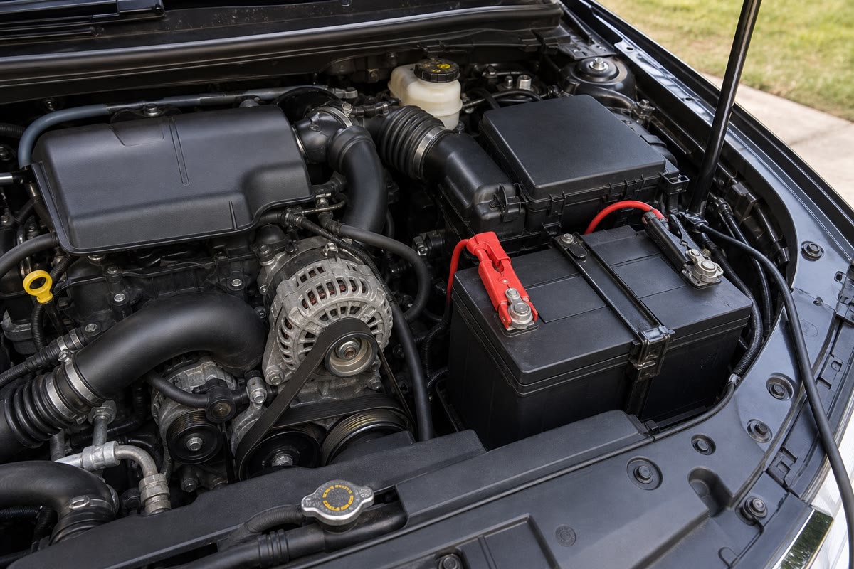
The battery is a real source, emf $E = 12.6\,\mathrm{V}$ , internal resistance $r = 10\,\mathrm{m}\Omega$ . Copper: $\rho = 1.7 \times 10^{-8}\,\Omega\,\mathrm{m}$ .

Part I — The battery alone.

Draw the Thévenin model and write $u(i)$ in the generator convention.
Give the open-circuit voltage and the short-circuit current. Why must a dropped wrench never bridge the terminals?
Write the Norton model of the same battery.
The battery feeds a resistor $R$ : express the current, the terminal voltage, the power $P_R$ delivered and the power lost in $r$ .
Show that $P_R$ is maximal for $R = r$ and compute that maximum. What is the efficiency then?
A technician measures $u = 12.48\,\mathrm{V}$ at $12\,\mathrm{A}$ and $u = 11.40\,\mathrm{V}$ at $120\,\mathrm{A}$ . Check that both points lie on the model and explain how a series of such points gives $E$ and $r$ by a straight-line fit.
The battery stores $60\,\mathrm{A}\,\mathrm{h}$ . How long could it run the two $55\,\mathrm{W}$ headlights alone (take $12\,\mathrm{V}$ )? How much energy is that in joules?

Part II — Cranking with the lights on. The starter is a resistor $R_s = 80\,\mathrm{m}\Omega$ ; each headlight is rated $55\,\mathrm{W}$ at $12.0\,\mathrm{V}$ and is treated as a resistor.

Compute the resistance of one headlight and of the two in parallel.
Starter alone: current, terminal voltage, power in the starter, power lost in the battery.
Starter and both headlights together: equivalent load resistance, total current, terminal voltage.
Use the current divider to find the starter current and the headlight current.
Compute the power each headlight now receives and compare with its rating: by what fraction do the lights dim?
Explain in two sentences, using the loop law, why the lights dim precisely because the starter draws a large current.
Would thicker battery cables help the lights? Justify qualitatively now (Part IV quantifies).

Part III — Engine running: the alternator. The alternator is a second real source, $E_a = 14.2\,\mathrm{V}$ , $r_a = 50\,\mathrm{m}\Omega$ , in parallel with the battery; the starter is off and both headlights are on.

Draw the circuit: two real sources and the headlight load in parallel between the same two nodes.
Apply Millman’s theorem to find the common terminal voltage.
Deduce the alternator current, the battery current (sign!) and the headlight current; check the node law.
Is the battery charging or discharging? What power does it receive, and what power does the alternator supply?
Recover the terminal voltage by superposition (each source alone, the other replaced by its internal resistance) and check.

Part IV — Sensors and wires.

The coolant sensor is a thermistor whose resistance falls from $2.0\,\mathrm{k}\Omega$ at $20{}^{\circ}\mathrm{C}$ to $300\,\Omega$ at $90{}^{\circ}\mathrm{C}$ ; it is the lower resistor of a divider fed by $5.0\,\mathrm{V}$ , the upper resistor being $R_0$ . Express the output voltage, and compute it at both temperatures for $R_0 = 775\,\Omega$ .
Show that the output swing between the two temperatures is largest when $R_0$ is the geometric mean of the two sensor values, and check the value above.
The same sensor is put in a Wheatstone bridge with three $775\,\Omega$ resistors: write the bridge output and say at what temperature it is balanced.
The starter cable is $1.5\,\mathrm{m}$ long each way. Compute the resistance of one conductor of cross-section $16\,\mathrm{mm}^{2}$ , the total voltage drop at $140\,\mathrm{A}$ , and the power dissipated in the cables.
Same with $4\,\mathrm{mm}^{2}$ cable: why is starter cable so thick?
Summarize: give the terminal voltage during cranking, the fraction of power reaching the starter, and the one law that explains the dimming of the lights.

Solution

Solution of Problem 6.1.

1. Ideal emf $E$ in series with $r$ : $u = E - ri$ .

2. $u(0) = 12.6\,\mathrm{V}$ ; $I_N = E/r = 1260\,\mathrm{A}$ . A wrench across the terminals would carry it: $16\,\mathrm{kW}$ in a few grams of steel — it melts and sprays.

3. Current source $I_N = 1260\,\mathrm{A}$ in parallel with $10\,\mathrm{m}\Omega$ .

4. $i = E/(R + r)$ ; $u = ER/(R + r)$ ; $P_R = E^2R/(R + r)^2$ ; $P_r = E^2r/(R + r)^2$ .

5. $\dd P_R/\dd R \propto (r - R)$ : maximum at $R = r$ , $P_{\max} = E^2/4r = 12.6^2/0.040 = 4.0\,\mathrm{kW}$ ; efficiency $R/(R + r) = 50\%$ .

6. $12.6 - 0.010 \times 12 = 12.48\,\mathrm{V}$ ; $12.6 - 0.010 \times 120 = 11.40\,\mathrm{V}$ . Plotting $u$ against $i$ gives a straight line of intercept $E$ and slope $-r$ (least squares, Chapter 1).

7. Two lamps: $110\,\mathrm{W}$ at $12\,\mathrm{V}$ , $9.2\,\mathrm{A}$ ; $60/9.2 = 6.5\,\mathrm{h}$ . Energy $60 \times 3600 \times 12 = 2.6\,\mathrm{MJ}$ .

8. $R_h = 12^2/55 = 2.62\,\Omega$ ; in parallel $1.31\,\Omega$ .

9. $i = 12.6/0.090 = 140\,\mathrm{A}$ ; $u = 12.6 - 1.4 = 11.2\,\mathrm{V}$ ; $P_s = 0.080 \times 140^2 = 1.57\,\mathrm{kW}$ ; lost $0.010 \times 140^2 = 196\,\mathrm{W}$ .

10. $R = 0.080 \parallel 1.31 = 75.4\,\mathrm{m}\Omega$ ; $i = 12.6/0.0854 = 148\,\mathrm{A}$ ; $u = 12.6 - 1.48 = 11.1\,\mathrm{V}$ .

11. $i_s = i \times 1.31/(1.31 + 0.080) = 139\,\mathrm{A}$ ; $i_h = 8.5\,\mathrm{A}$ for the two lamps.

12. Each lamp: $u^2/R_h = 11.1^2/2.62 = 47\,\mathrm{W}$ against $55\,\mathrm{W}$ : down by $14\%$ .

13. Loop law: the terminal voltage is $u = E - ri$ ; the starter’s $140\,\mathrm{A}$ produces a $1.4\,\mathrm{V}$ drop inside the battery, and the lamps, in parallel on the same terminals, receive that reduced voltage.

14. Only partly: thicker cables cut the drop in the cables, not in $r$ ; lamps fed from the battery terminals still see $E - ri$ .

15. Three branches between the same two nodes: $(E, r)$ , $(E_a, r_a)$ and $R_h = 1.31\,\Omega$ .

16. $V = \dfrac{12.6/0.010 + 14.2/0.050 + 0/1.31}{100 + 20 + 0.763} = \dfrac{1544}{120.8} = 12.79\,\mathrm{V}$ .

17. Alternator $(14.2 - 12.79)/0.050 = 28.3\,\mathrm{A}$ ; battery $(12.6 - 12.79)/0.010 = -18.6\,\mathrm{A}$ (flowing into it); lamps $12.79/1.31 = 9.8\,\mathrm{A}$ ; $28.3 = 18.6 + 9.8$ .

18. Charging. It receives $12.79 \times 18.6 = 238\,\mathrm{W}$ ( $234\,\mathrm{W}$ stored, $3.5\,\mathrm{W}$ heat); the alternator supplies $12.79 \times 28.3 = 362\,\mathrm{W}$ at its terminals.

19. Battery alone (alternator $\to$ $50\,\mathrm{m}\Omega$ ): load $0.050 \parallel 1.31 = 48.2\,\mathrm{m}\Omega$ , $u_1 = 12.6 \times 48.2/58.2 = 10.44\,\mathrm{V}$ . Alternator alone (battery $\to$ $10\,\mathrm{m}\Omega$ ): load $0.010 \parallel 1.31 = 9.92\,\mathrm{m}\Omega$ , $u_2 = 14.2 \times 9.92/59.9 = 2.35\,\mathrm{V}$ . Sum $12.79\,\mathrm{V}$ .

20. $u = 5.0\,R_s/(R_0 + R_s)$ : $3.60\,\mathrm{V}$ at $20{}^{\circ}\mathrm{C}$ , $1.40\,\mathrm{V}$ at $90{}^{\circ}\mathrm{C}$ .

21. $\Delta u = 5[R_a/(R_0 + R_a) - R_b/(R_0 + R_b)]$ ; $\dd\Delta u/\dd R_0 = 0 \Leftrightarrow R_a/(R_0 + R_a)^2 = R_b/(R_0 + R_b)^2 \Leftrightarrow R_0^2 = R_aR_b$ : $R_0 = \sqrt{2000 \times 300} = 775\,\Omega$ .

22. $u = 5[\tfrac12 - R_s/(775 + R_s)]$ , zero when $R_s = 775\,\Omega$ , i.e. at the mid-range temperature where the thermistor reaches that value.

23. $R = 1.7\times10^{-8} \times 1.5/16\times10^{-6} = 1.6\,\mathrm{m}\Omega$ per conductor, $3.2\,\mathrm{m}\Omega$ total; drop $0.0032 \times 140 = 0.45\,\mathrm{V}$ ; power $63\,\mathrm{W}$ .

24. $4\,\mathrm{mm}^{2}$ : $6.4\,\mathrm{m}\Omega$ each, $12.8\,\mathrm{m}\Omega$ total: drop $1.8\,\mathrm{V}$ , $250\,\mathrm{W}$ wasted — the starter would lose a sixth of its voltage. Thick cable keeps $R_{\text{cable}} \ll R_s$ .

25. About $11.1\,\mathrm{V}$ at the terminals during cranking; the starter receives $1568/(1568 + 196) \approx 89\%$ of the battery’s power; the dimming is the loop law, $u = E - ri$ .

Terms defined in this chapter

See all 393 terms in the glossary