University Physics — Year 1 · Bachelor Year 1

7Transient Regimes: First and Second Order

Push down on the corner of a parked car and let go. A car in good order rises once and stops; a car with worn shock absorbers bobs two or three times before it settles. In an electronics lab the same two behaviors appear on an oscilloscope when a capacitor discharges through a coil: a smooth return, or a ringing that dies out. Both are the transient between one steady state and another, and both obey the same small family of linear differential equations — first order for a single energy store, second order for two that exchange. This chapter solves them once and for all, names their parameters (time constant, natural frequency, quality factor), and shows how the same numbers describe a circuit and a suspension.

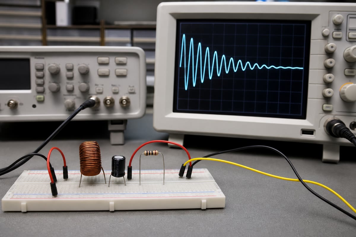
A coil, a capacitor and a resistor on a breadboard, and on the oscilloscope the decaying oscillation that follows a step: the pseudo-periodic regime of this chapter.

7.1 First-order systems

Definition 7.1 (First-order linear system)

A quantity $x(t)$ obeys a first-order linear equation with constant coefficients when

\tau\,\frac{\dd x}{\dd t} + x = x_\infty ,

with $\tau > 0$ the time constant and $x_\infty$ a constant (the value imposed by the source). Its steady state is $x = x_\infty$ ; the transient regime is the approach to it from the initial value $x(0) = x_0$ .

Theorem 7.2 (Solution)

The unique solution with $x(0) = x_0$ is

x(t) = x_\infty + (x_0 - x_\infty)\,\eu^{-t/\tau} .

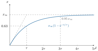
The gap to the steady state shrinks by the factor $\eu^{-1} \approx 0.37$ every $\tau$ : $63\%$ of the way at $\tau$ , $95\%$ at $3\tau$ , $99\%$ at $4.6\tau$ . The tangent at the origin reaches $x_\infty$ at $t = \tau$ .

Proof. $y = x - x_\infty$ obeys $\tau y' + y = 0$ , whose solutions are $y = K\eu^{-t/\tau}$ (the mathematics course on linear differential equations proves there are no others); $K = x_0 - x_\infty$ . The slope at $0$ is $-(x_0 - x_\infty)/\tau$ , which would close the gap in time $\tau$ . ∎

The first-order step response from x_0 = 0: the initial tangent meets the asymptote at t =; 63\% of the way at , 95\% at 3. Every first-order transient is this curve, stretched by and shifted by x_0 and x_∈fty. — The first-order step response from $x_0 = 0$ : the initial tangent meets the asymptote at $t = \tau$ ; $63\%$ of the way at $\tau$ , $95\%$ at $3\tau$ . Every first-order transient is this curve, stretched by $\tau$ and shifted by $x_0$ and $x_\infty$ .

Proposition 7.3 (RC and RL circuits)

A capacitor $C$ charged through a resistor $R$ from an ideal source $E$ obeys $RC\,\dd u_C/\dd t + u_C = E$ : $\tau = RC$ , $u_{C,\infty} = E$ . A coil $L$ in series with $R$ across $E$ obeys $(L/R)\,\dd i/\dd t + i = E/R$ : $\tau = L/R$ , $i_\infty = E/R$ . With the source removed ( $E \to 0$ ) the same equations describe the discharge toward zero.

Proof. Loop law $E = Ri + u_C$ with $i = C\,\dd u_C/\dd t$ ; loop law $E = Ri + L\,\dd i/\dd t$ . ∎

Proposition 7.4 (Continuity conditions)

The voltage across a capacitor and the current through an inductor are continuous functions of time: at a switching instant $t_0$ , $u_C(t_0^+) = u_C(t_0^-)$ and $i_L(t_0^+) = i_L(t_0^-)$ . Currents in resistors and voltages across coils may jump.

Proof. A jump of $u_C$ would require $i = C\,\dd u_C/\dd t$ infinite, a jump of $i_L$ would require $u = L\,\dd i/\dd t$ infinite; both are impossible in a circuit of finite voltages and currents (equivalently, the stored energies $\tfrac12 Cu_C^2$ and $\tfrac12 Li^2$ cannot change instantaneously without infinite power). ∎

Method 7.5 (Solving a first-order transient)

Write the loop and node laws after the switch, with the component laws; reduce to one equation in $u_C$ or $i_L$ and put it in the form $\tau x' + x = x_\infty$ ; read $\tau$ and $x_\infty$ (the latter is also the steady state found by replacing $C$ by an open circuit, $L$ by a wire).
Find $x_0$ from the continuity of $u_C$ or $i_L$ across the switching instant, using the circuit before it.
Write $x = x_\infty + (x_0 - x_\infty)\eu^{-t/\tau}$ ; deduce the other quantities by differentiation and the loop law.

When the capacitor sees a network of resistors and sources, replace that network by its Thévenin equivalent $(E_{\mathrm{Th}}, R_{\mathrm{Th}})$ first (Chapter 6): $\tau = R_{\mathrm{Th}}C$ , $u_\infty = E_{\mathrm{Th}}$ .

Proposition 7.6 (Energy balance of the RC charge)

Charging a capacitor from $0$ to $E$ through any resistor $R$ , the source supplies $CE^2$ , the capacitor stores $\tfrac12 CE^2$ , and the resistor dissipates the other $\tfrac12 CE^2$ — whatever $R$ .

Proof. $i = (E/R)\eu^{-t/\tau}$ ; the source supplies $\int_0^\infty Ei\,\dd t = E \cdot (E/R)\tau = CE^2$ ; the resistor takes $\int_0^\infty Ri^2\,\dd t = (E^2/R)\int_0^\infty \eu^{-2t/\tau}\dd t = (E^2/R)(\tau/2) = \tfrac12 CE^2$ ; the difference is the stored $\tfrac12 CE^2$ . A smaller $R$ dissipates the same energy faster. ∎

Example 7.7 (A relay coil)

$L = 20\,\mathrm{mH}$ , $R = 5.0\,\Omega$ , $E = 10\,\mathrm{V}$ : $\tau = 4.0\,\mathrm{ms}$ , $i_\infty = 2.0\,\mathrm{A}$ ; the contacts pull in when $i$ reaches $1.5\,\mathrm{A}$ , i.e. at $t = -\tau\ln(1 - 0.75) = 5.5\,\mathrm{ms}$ . Opening the circuit, $i$ must fall from $2\,\mathrm{A}$ ; a “freewheeling” diode across the coil gives it a path through $R$ alone, $\tau = 4\,\mathrm{ms}$ , instead of a spark.

7.2 Second-order systems

Definition 7.8 (Canonical second-order form)

A quantity $x(t)$ is a second-order linear system when

\frac{\dd^2 x}{\dd t^2} + \frac{\omega_0}{Q}\,\frac{\dd x}{\dd t} + \omega_0^2\,x = \omega_0^2\,x_\infty ,

with $\omega_0 > 0$ the natural angular frequency, $Q > 0$ the quality factor (dimensionless), and $x_\infty$ the steady state. One also writes $\omega_0/Q = 2\xi\omega_0$ with $\xi = 1/2Q$ the damping ratio.

Proposition 7.9 (The series RLC circuit)

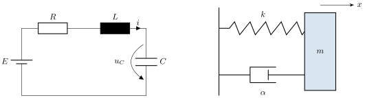
A capacitor $C$ , a coil $L$ and a resistor $R$ in series across a source $E$ : the capacitor voltage obeys the canonical form with

\omega_0 = \frac{1}{\sqrt{LC}}, \qquad Q = \frac{1}{R}\sqrt{\frac{L}{C}}, \qquad u_{C,\infty} = E .

Proof. Loop law: $E = L\,\dd i/\dd t + Ri + u_C$ with $i = C\,\dd u_C/\dd t$ : $LC\,u_C'' + RC\,u_C' + u_C = E$ ; divide by $LC$ and identify $\omega_0^2 = 1/LC$ , $\omega_0/Q = R/L$ . ∎

The two faces of the second-order system: the series RLC circuit (_0 = 1/√LC, Q = √L/C/R) and the mass–spring–damper (_0 = √k/m, Q = √km/). Same equation, same three regimes. — The two faces of the second-order system: the series RLC circuit ( $\omega_0 = 1/\sqrt{LC}$ , $Q = \sqrt{L/C}/R$ ) and the mass–spring–damper ( $\omega_0 = \sqrt{k/m}$ , $Q = \sqrt{km}/\alpha$ ). Same equation, same three regimes.

Proposition 7.10 (The mechanical oscillator)

A mass $m$ on a spring of stiffness $k$ with a viscous damper of coefficient $\alpha$ (force $-\alpha\dot x$ ), displaced by $x$ from equilibrium, obeys $m\ddot x + \alpha\dot x + kx = 0$ : the canonical form with

\omega_0 = \sqrt{\frac{k}{m}}, \qquad Q = \frac{\sqrt{km}}{\alpha} .

The correspondence $x \leftrightarrow q$ , $\dot x \leftrightarrow i$ , $m \leftrightarrow L$ , $\alpha \leftrightarrow R$ , $k \leftrightarrow 1/C$ maps every result of one system onto the other.

Proof. Newton’s second law (Chapter 12) with the spring force $-kx$ and the damping force; divide by $m$ . ∎

Theorem 7.11 (The three regimes)

The solutions of the homogeneous equation $x'' + (\omega_0/Q)x' + \omega_0^2 x = 0$ are governed by the roots of $r^2 + (\omega_0/Q)r + \omega_0^2 = 0$ , of discriminant $\Delta = \omega_0^2(1/Q^2 - 4)$ :

$Q < \tfrac12$ , aperiodic: two real negative roots $r_\pm = -\frac{\omega_0}{2Q}\big(1 \mp \sqrt{1 - 4Q^2}\big)$ , $x = A\eu^{r_+t} + B\eu^{r_-t}$ , a return without oscillation;
$Q = \tfrac12$ , critical: a double root $r = -\omega_0$ , $x = (A + Bt)\eu^{-\omega_0 t}$ , the fastest return without overshoot;
$Q > \tfrac12$ , pseudo-periodic: complex roots $r = -1/\tau \pm \iu\omega$ with

$\tau = \frac{2Q}{\omega_0}, \qquad \omega = \omega_0\sqrt{1 - \frac{1}{4Q^2}}, \qquad x = \eu^{-t/\tau}\big(A\cos\omega t + B\sin\omega t\big),$

a damped oscillation of pseudo-period $T = 2\pi/\omega$ inside the envelope $\pm\sqrt{A^2 + B^2}\,\eu^{-t/\tau}$ .

The full solution with a constant right-hand side is $x_\infty$ plus the homogeneous solution; $A$ and $B$ follow from $x(0)$ and $x'(0)$ .

Proof. Characteristic equation of a linear equation with constant coefficients (mathematics course, second-order linear equations): the roots are $r = -\omega_0/2Q \pm \tfrac12\sqrt\Delta$ . For $Q > \tfrac12$ , $\sqrt\Delta = \iu\omega_0\sqrt{4 - 1/Q^2}$ , giving the real part $-\omega_0/2Q = -1/\tau$ and the imaginary part $\pm\omega_0\sqrt{1 - 1/4Q^2}$ ; the real solutions are the combinations of $\eu^{-t/\tau}\cos\omega t$ and $\eu^{-t/\tau}\sin\omega t$ . ∎

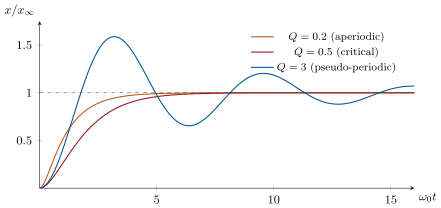
Step response of a second-order system from rest, for three quality factors. Small Q: a slow creep; Q = 1/2: the quickest return without overshoot; large Q: ringing that lasts about Q oscillations. — Step response of a second-order system from rest, for three quality factors. Small $Q$ : a slow creep; $Q = \tfrac12$ : the quickest return without overshoot; large $Q$ : ringing that lasts about $Q$ oscillations.

Proposition 7.12 (Reading $Q$ on a pseudo-periodic trace)

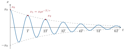
In the pseudo-periodic regime, two successive maxima are in the ratio $x_{n+1}/x_n = \eu^{-T/\tau}$ ; the logarithmic decrement

\delta = \ln\frac{x_n}{x_{n+1}} = \frac{T}{\tau} = \frac{\pi}{Q\sqrt{1 - 1/4Q^2}} \approx \frac{\pi}{Q} \quad (Q \gg 1)

gives $Q$ ; the number of oscillations visible before the amplitude falls below $5\%$ is about $Q$ . For $Q \gg 1$ , $\omega \approx \omega_0$ and $T \approx 2\pi/\omega_0$ .

Proof. The envelope $\eu^{-t/\tau}$ multiplies by $\eu^{-T/\tau}$ per period; $T/\tau = (2\pi/\omega)(\omega_0/2Q)$ . The envelope reaches $\eu^{-3} \approx 5\%$ at $3\tau = 6Q/\omega_0 \approx Q\,T$ , i.e. after about $Q$ periods. ∎

Free pseudo-periodic decay, x = x_0 -t/ t: successive maxima shrink by the constant factor -T/, and (x_n/x_n+1) = T/ π/Q measures the quality factor from the trace. — Free pseudo-periodic decay, $x = x_0\eu^{-t/\tau}\cos\omega t$ : successive maxima shrink by the constant factor $\eu^{-T/\tau}$ , and $\ln(x_n/x_{n+1}) = T/\tau \approx \pi/Q$ measures the quality factor from the trace.

Example 7.13 (An RLC ringing)

$L = 10\,\mathrm{mH}$ , $C = 100\,\mathrm{nF}$ , $R = 100\,\Omega$ : $\omega_0 = 1/\sqrt{10^{-9}} = 3.16 \times 10^{4}\,\mathrm{rad}/\mathrm{s}$ ( $f_0 = 5.03\,\mathrm{kHz}$ ), $Q = \sqrt{L/C}/R = 316/100 = 3.16$ : pseudo-periodic, $\tau = 2Q/\omega_0 = 0.20\,\mathrm{ms}$ , $\omega = 0.987\,\omega_0$ , $T = 0.20\,\mathrm{ms}$ , three visible oscillations. The critical resistance is $R_c = 2\sqrt{L/C} = 632\,\Omega$ ; above it the discharge is aperiodic.

Method 7.14 (Solving a second-order transient)

Write the equation; put it in canonical form; read $\omega_0$ , $Q$ and $x_\infty$ .
Decide the regime from $Q$ and write the general solution as $x_\infty$ plus the homogeneous solution.
Find $x(0)$ and $x'(0)$ from the continuity of $u_C$ and $i_L$ (for the RLC: $u_C(0^+) = u_C(0^-)$ and $u_C'(0^+) = i(0^-)/C$ ); solve for the two constants.

Example 7.15 (Initial conditions)

The capacitor of the previous example is charged to $U_0$ and, at $t = 0$ , closed on $L$ and $R$ (no source): $x_\infty = 0$ , $u_C(0) = U_0$ , $u_C'(0) = i(0)/C = 0$ since the coil current was zero. Hence $A = U_0$ and $-A/\tau + B\omega = 0$ , $B = U_0/(\omega\tau) = U_0/\sqrt{4Q^2 - 1}$ : $u_C = U_0\eu^{-t/\tau}[\cos\omega t + \sin(\omega t)/\sqrt{4Q^2 - 1}]$ — for $Q \gg 1$ simply $U_0\eu^{-t/\tau}\cos\omega_0 t$ , and the current $i = -C\,\dd u_C/\dd t$ peaks near $U_0\sqrt{C/L} = U_0/(\omega_0 L)$ .

Remark 7.16 (Energy)

The stored energy $\tfrac12 Cu_C^2 + \tfrac12 Li^2$ (or $\tfrac12 kx^2 + \tfrac12 m\dot x^2$ ) decreases at the rate $Ri^2$ ( $\alpha\dot x^2$ ): differentiate and use the equation. Each pseudo-period the energy shrinks by the factor $\eu^{-2T/\tau}$ ; with $Q = 3$ about $88\%$ of it is lost per oscillation. A high $Q$ means a slow leak relative to the oscillation — a good clock, a sharp resonance (Chapter 8) — and a low $Q$ a quick return: the right choice for a suspension or a meter needle.

7.3 Exercises

Exercise 7.1 ★

An RC circuit: $R = 10\,\mathrm{k}\Omega$ , $C = 47\,\mathrm{nF}$ , charged from $E$ . Compute $\tau$ , $u_C(\tau)/E$ , and the time to reach $99\%$ of $E$ .

Solution

Solution of Exercise 7.1.

$\tau = RC = 10^4 \times 47\times10^{-9} = 0.47\,\mathrm{ms}$ ; $u_C(\tau)/E = 1 - \eu^{-1} = 0.63$ ; $99\%$ : $\eu^{-t/\tau} = 0.01$ , $t = \tau\ln 100 = 4.6\tau = 2.2\,\mathrm{ms}$ .

Exercise 7.2 ★

An RL circuit: $L = 20\,\mathrm{mH}$ , $R = 5.0\,\Omega$ , $E = 10\,\mathrm{V}$ . Compute $\tau$ , the final current, the current at $t = \tau$ , and the voltage across the coil just after closing the switch.

Solution

Solution of Exercise 7.2.

$\tau = L/R = 4.0\,\mathrm{ms}$ ; $i_\infty = E/R = 2.0\,\mathrm{A}$ ; $i(\tau) = 0.63 \times 2.0 = 1.26\,\mathrm{A}$ ; at $0^+$ , $i = 0$ (continuity), so $u_L = E - Ri = 10\,\mathrm{V}$ .

Exercise 7.3 ★

A series RLC: $L = 10\,\mathrm{mH}$ , $C = 100\,\mathrm{nF}$ , $R = 100\,\Omega$ . Compute $\omega_0$ , $f_0$ , $Q$ ; name the regime; give $\tau$ and the pseudo-period.

Solution

Solution of Exercise 7.3.

$\omega_0 = 1/\sqrt{LC} = 3.16 \times 10^{4}\,\mathrm{rad}/\mathrm{s}$ , $f_0 = 5.03\,\mathrm{kHz}$ ; $Q = \sqrt{L/C}/R = 316/100 = 3.2 > \tfrac12$ : pseudo-periodic; $\tau = 2Q/\omega_0 = 0.20\,\mathrm{ms}$ ; $\omega = \omega_0\sqrt{1 - 1/4Q^2} = 0.987\omega_0$ , $T = 0.20\,\mathrm{ms}$ .

Exercise 7.4 ★

For the same $L$ and $C$ , what resistance gives the critical regime? What is $Q$ then? What happens for $R = 2\,\mathrm{k}\Omega$ ?

Solution

Solution of Exercise 7.4.

$R_c = 2\sqrt{L/C} = 632\,\Omega$ , $Q = \tfrac12$ . At $2\,\mathrm{k}\Omega$ , $Q = 0.16$ : aperiodic, a slow creep governed by the small root $\abs{r_+} \approx \omega_0 Q = 5 \times 10^{3}\,\mathrm{s}^{-1}$ (time scale $0.2\,\mathrm{ms}$ but no oscillation).

Exercise 7.5 ★★

A charged capacitor $C = 1.0\,\text{µ}\mathrm{F}$ discharges through an unknown $R$ ; the voltage halves every $3.5\,\mathrm{ms}$ . Show that the half-life is $\tau\ln 2$ and find $R$ .

Solution

Solution of Exercise 7.5.

$u = U_0\eu^{-t/\tau}$ halves when $\eu^{-t/\tau} = \tfrac12$ : $t_{1/2} = \tau\ln 2$ . $\tau = 3.5/0.693 = 5.05\,\mathrm{ms}$ , $R = \tau/C = 5.1\,\mathrm{k}\Omega$ .

Exercise 7.6 ★★

Show by direct integration that charging a capacitor from $0$ to $E$ through $R$ dissipates exactly $\tfrac12 CE^2$ in $R$ , independently of $R$ . What becomes of the efficiency of the transfer, and how could one do better?

Solution

Solution of Exercise 7.6.

$i = (E/R)\eu^{-t/\tau}$ : $\int_0^\infty Ri^2\,\dd t = (E^2/R)(\tau/2) = \tfrac12 CE^2$ , no $R$ in sight. The source supplies $CE^2$ : efficiency $50\%$ for any resistor. Better: charge through an inductor (the current is then not proportional to the voltage gap) or in several voltage steps — each step of $E/n$ loses only $\tfrac12 C(E/n)^2$ .

Exercise 7.7 ★★

On an oscilloscope, a free RLC decay shows successive maxima of $2.0\,\mathrm{V}$ , $1.5\,\mathrm{V}$ , $1.12\,\mathrm{V}$ at intervals of $0.40\,\mathrm{ms}$ . Deduce $Q$ , $\omega_0$ , and, with $C = 1.0\,\text{µ}\mathrm{F}$ , the values of $L$ and $R$ .

Solution

Solution of Exercise 7.7.

$\delta = \ln(2.0/1.5) = 0.29$ (and $\ln(1.5/1.12) = 0.29$ : consistent); $Q \approx \pi/\delta = 11$ . $T = 0.40\,\mathrm{ms}$ , so $\omega_0 \approx 2\pi/T = 1.57 \times 10^{4}\,\mathrm{rad}/\mathrm{s}$ (the correction $1/8Q^2$ is $0.1\%$ ). $L = 1/(\omega_0^2 C) = 4.1\,\mathrm{mH}$ ; $R = \omega_0 L/Q = 5.8\,\Omega$ .

Exercise 7.8 ★★

A capacitor charged to $U_0 = 100\,\mathrm{V}$ ( $C = 10\,\text{µ}\mathrm{F}$ ) is switched onto a coil $L = 1.0\,\mathrm{mH}$ of small resistance ( $Q \gg 1$ ). Write $u_C(t)$ and $i(t)$ , and estimate the peak current. Where does the energy sit at the peak?

Solution

Solution of Exercise 7.8.

$u_C \approx U_0\eu^{-t/\tau}\cos\omega_0 t$ ; $i = -C\,\dd u_C/\dd t \approx CU_0\omega_0\sin\omega_0 t$ (for $t \ll \tau$ ), peak $U_0\sqrt{C/L} = 100 \times 0.1 = 10\,\mathrm{A}$ , reached a quarter period after closing, when $u_C = 0$ : all the energy ( $\tfrac12 CU_0^2 = 50\,\mathrm{mJ}$ ) is then magnetic, $\tfrac12 Li^2 = 50\,\mathrm{mJ}$ .

Exercise 7.9 ★★

A quarter of a car: $m = 400\,\mathrm{kg}$ on a spring $k = 2.0 \times 10^{4}\,\mathrm{N}/\mathrm{m}$ . Compute $\omega_0$ , $f_0$ and the critical damping coefficient. With a damper $\alpha = 2000\,\mathrm{N}\,\mathrm{s}/\mathrm{m}$ , give $Q$ , the regime, the pseudo-period and the decay time $\tau$ .

Solution

Solution of Exercise 7.9.

$\omega_0 = \sqrt{k/m} = 7.1\,\mathrm{rad}/\mathrm{s}$ , $f_0 = 1.1\,\mathrm{Hz}$ ; $\alpha_c = 2\sqrt{km} = 2\sqrt{8\times10^6} = 5.7 \times 10^{3}\,\mathrm{N}\,\mathrm{s}/\mathrm{m}$ . $\alpha = 2000$ : $Q = \sqrt{km}/\alpha = 2828/2000 = 1.4$ , pseudo-periodic; $T = 2\pi/(\omega_0\sqrt{1 - 1/4Q^2}) = 0.89/0.935 = 0.95\,\mathrm{s}$ ; $\tau = 2Q/\omega_0 = 0.40\,\mathrm{s}$ .

Exercise 7.10 ★★★

A coil $L = 0.50\,\mathrm{H}$ carries $I_0 = 2.0\,\mathrm{A}$ ; the source is disconnected and the coil is left on a bleed resistor $R = 100\,\Omega$ . Give $i(t)$ , $\tau$ , the peak voltage across the coil and the energy dissipated. What would happen without the resistor?

Solution

Solution of Exercise 7.10.

$i = I_0\eu^{-t/\tau}$ , $\tau = L/R = 5.0\,\mathrm{ms}$ ; peak voltage $RI_0 = 200\,\mathrm{V}$ at $t = 0^+$ ; energy $\tfrac12 LI_0^2 = 1.0\,\mathrm{J}$ dissipated in $R$ . Without the resistor the current has no path: $\dd i/\dd t$ is huge, the coil voltage reaches kilovolts, and an arc jumps the switch.

Exercise 7.11 ★★★

A capacitor $C = 1.0\,\text{µ}\mathrm{F}$ is charged from $E = 12\,\mathrm{V}$ through $R_1 = 10\,\mathrm{k}\Omega$ while $R_2 = 20\,\mathrm{k}\Omega$ is connected across it. Using a Thévenin equivalent, find the time constant and the final voltage; write $u_C(t)$ from $u_C(0) = 0$ .

Solution

Solution of Exercise 7.11.

Seen from $C$ : $E_{\mathrm{Th}} = ER_2/(R_1 + R_2) = 8.0\,\mathrm{V}$ , $R_{\mathrm{Th}} = R_1 \parallel R_2 = 6.67\,\mathrm{k}\Omega$ ; $\tau = R_{\mathrm{Th}}C = 6.7\,\mathrm{ms}$ ; $u_C = 8.0(1 - \eu^{-t/\tau})$ V.

Exercise 7.12 ★★★

Critical regime, step from rest ( $x(0) = x'(0) = 0$ ): show that $x = x_\infty[1 - (1 + \omega_0 t)\eu^{-\omega_0 t}]$ , and find numerically the time to reach $95\%$ of $x_\infty$ (in units of $1/\omega_0$ ). Compare with the settling time of the envelope for $Q = 5$ and for the slow root when $Q = 0.1$ ; conclude on why “critical” is the engineer’s target.

Solution

Solution of Exercise 7.12.

Double root $-\omega_0$ : $x = x_\infty + (A + Bt)\eu^{-\omega_0 t}$ ; $x(0) = 0$ gives $A = -x_\infty$ , $x'(0) = 0$ gives $B = \omega_0 A$ : $x = x_\infty[1 - (1 + \omega_0 t)\eu^{-\omega_0 t}]$ . $95\%$ : $(1 + s)\eu^{-s} = 0.05$ , $s \approx 4.7$ : $t_{95} = 4.7/\omega_0$ . For $Q = 5$ the envelope $\eu^{-t/\tau}$ with $\tau = 10/\omega_0$ needs $3\tau = 30/\omega_0$ ; for $Q = 0.1$ the slow root is $\abs{r_+} \approx \omega_0 Q$ and $3/\abs{r_+} = 30/\omega_0$ . Both are six times slower: critical damping is the fastest no-overshoot return, which is what a meter, a door closer or a suspension wants.

7.4 Problem: Designing a suspension

Problem 7.1

Weekend problem — the same differential equation on a lab bench and under a car: how many bounces a worn shock absorber allows, what the designer chooses instead, and how one number tells the two apart

Part I studies a series RLC circuit, $L = 10\,\mathrm{mH}$ , $C = 100\,\mathrm{nF}$ ; Parts II–IV a quarter-car model: a mass $m = 350\,\mathrm{kg}$ resting on a spring $k = 22\,\mathrm{kN}/\mathrm{m}$ and a shock absorber exerting $-\alpha\dot x$ . Overshoot of a step response in the pseudo-periodic regime (given): $x_{\max}/x_\infty - 1 = \exp(-\pi\xi/\sqrt{1 - \xi^2})$ , $\xi = 1/2Q$ .

Part I — The circuit.

Write the loop law for the series RLC across a source $E$ , and the differential equation for $u_C$ .
Put it in canonical form; express $\omega_0$ and $Q$ .
Compute $\omega_0$ , $f_0$ and the critical resistance $R_c$ .
Write the characteristic equation and its discriminant; state the three regimes in terms of $Q$ .
In the pseudo-periodic case, give $\tau$ and $\omega$ and the form of $u_C(t)$ .
For $R = 100\,\Omega$ compute $Q$ , $\tau$ , the pseudo-period, and the number of visible oscillations.
The capacitor, charged to $U_0$ , is switched onto $L$ and $R$ at $t = 0$ . Give $u_C(0^+)$ and $\dd u_C/\dd t(0^+)$ , with the physical reason for each.

Part II — The quarter car.

Measuring $x$ from the equilibrium position, write Newton’s second law for the body and show that weight drops out.
Put the equation in canonical form; give $\omega_0$ and $Q$ in terms of $m$ , $k$ , $\alpha$ , and list the electromechanical correspondences.
Compute $\omega_0$ , $f_0$ and the critical coefficient $\alpha_c$ .
The designer fits $\alpha = 4000\,\mathrm{N}\,\mathrm{s}/\mathrm{m}$ : compute $Q$ , $\xi$ , and name the regime.
Compute $\tau$ and the pseudo-period.
Compute the overshoot after a step (a kerb): is the car comfortable?
What resistance $R$ would give the circuit of Part I the same $Q$ as this suspension?

Part III — The worn damper. Oil has leaked: $\alpha = 1200\,\mathrm{N}\,\mathrm{s}/\mathrm{m}$ .

Compute $Q$ , the pseudo-period and $\tau$ .
By what factor do successive maxima shrink? How many bounces are visible before the amplitude is below $5\%$ ?
The bounce test: one pushes the corner down by $x_0 = 5.0\,\mathrm{cm}$ and releases. Give the initial conditions, the energy stored in the spring, and say where that energy goes.
Estimate the peak velocity of the body during the first return ( $\approx x_0\omega_0$ for $Q \gg 1$ ) and the peak damper force.
Why is the exactly critical damping ( $Q = \tfrac12$ ) not the designer’s choice, although it gives no overshoot? (Think of the last few millimeters of the return.)
Compute the overshoot for the worn damper and compare with Part II.

Part IV — Diagnosing $Q$ from a trace. An accelerometer on the body records the free decay.

For the worn car, successive maxima read $1.00$ , $0.25$ , $0.062$ (arbitrary units). Compute the logarithmic decrement, deduce $\xi$ exactly from $\delta = 2\pi\xi/\sqrt{1 - \xi^2}$ , then $Q$ ; compare with Part III.
For the healthy car no second maximum is visible; only the overshoot, $3.8\%$ , can be read. Invert the overshoot formula to find $\xi$ and $Q$ .
What fraction of the mechanical energy does the worn damper dissipate per pseudo-period?
A technician who has no car at hand builds the RLC of Part I with $R$ chosen so that $Q = 2.3$ : what $R$ , and why is the oscilloscope trace, plotted against $\omega_0 t$ , identical in shape to the car’s?
Summarize: which dimensionless number decides the shape of any second-order transient, what value a suspension designer aims for, and what a driver should conclude from “more than one bounce”.

Solution

Solution of Problem 7.1.

1. $E = L\,\dd i/\dd t + Ri + u_C$ , $i = C\,\dd u_C/\dd t$ : $LC\,u_C'' + RC\,u_C' + u_C = E$ .

2. $u_C'' + (\omega_0/Q)u_C' + \omega_0^2u_C = \omega_0^2E$ with $\omega_0 = 1/\sqrt{LC}$ , $Q = \sqrt{L/C}/R$ .

3. $\omega_0 = 3.16 \times 10^{4}\,\mathrm{rad}/\mathrm{s}$ , $f_0 = 5.03\,\mathrm{kHz}$ , $R_c = 2\sqrt{L/C} = 632\,\Omega$ .

4. $r^2 + (\omega_0/Q)r + \omega_0^2 = 0$ , $\Delta = \omega_0^2(1/Q^2 - 4)$ : $Q < \tfrac12$ aperiodic, $Q = \tfrac12$ critical, $Q > \tfrac12$ pseudo-periodic.

5. $\tau = 2Q/\omega_0$ , $\omega = \omega_0\sqrt{1 - 1/4Q^2}$ , $u_C = E + \eu^{-t/\tau}(A\cos\omega t + B\sin\omega t)$ .

6. $Q = 3.16$ , $\tau = 0.20\,\mathrm{ms}$ , $T = 2\pi/\omega = 0.20\,\mathrm{ms}$ , about three oscillations.

7. $u_C(0^+) = U_0$ ( $u_C$ continuous: finite current); $u_C'(0^+) = i(0^+)/C = 0$ ( $i_L$ continuous and zero before).

8. $m\ddot x = -k(x + x_{\text{eq}}) - \alpha\dot x + mg$ with $kx_{\text{eq}} = mg$ : $m\ddot x + \alpha\dot x + kx = 0$ .

9. $\omega_0 = \sqrt{k/m}$ , $Q = \sqrt{km}/\alpha$ ; $x \leftrightarrow q$ , $\dot x \leftrightarrow i$ , $m \leftrightarrow L$ , $\alpha \leftrightarrow R$ , $k \leftrightarrow 1/C$ .

10. $\omega_0 = \sqrt{22000/350} = 7.93\,\mathrm{rad}/\mathrm{s}$ , $f_0 = 1.26\,\mathrm{Hz}$ ; $\alpha_c = 2\sqrt{km} = 5.55 \times 10^{3}\,\mathrm{N}\,\mathrm{s}/\mathrm{m}$ .

11. $Q = 2775/4000 = 0.69$ , $\xi = 0.72$ : pseudo-periodic, just under critical.

12. $\tau = 2Q/\omega_0 = 0.18\,\mathrm{s}$ ; $\omega = \omega_0\sqrt{1 - \xi^2} = 5.5\,\mathrm{rad}/\mathrm{s}$ , $T = 1.1\,\mathrm{s}$ .

13. Overshoot $\exp(-\pi \times 0.72/0.69) = \exp(-3.3) = 3.8\%$ : one small rise past equilibrium, then done — comfortable.

14. $R = \sqrt{L/C}/Q = 316/0.69 = 455\,\Omega$ .

15. $Q = 2775/1200 = 2.3$ , $\xi = 0.22$ ; $\omega = 0.976\omega_0$ , $T = 0.81\,\mathrm{s}$ ; $\tau = 2Q/\omega_0 = 0.58\,\mathrm{s}$ .

16. $\eu^{-T/\tau} = \eu^{-1.39} = 0.25$ : each bounce is a quarter of the previous; $0.25^3 = 1.6\%$ : three visible bounces.

17. $x(0) = -x_0$ , $\dot x(0) = 0$ ; energy $\tfrac12 kx_0^2 = 0.5 \times 22000 \times 0.0025 = 28\,\mathrm{J}$ , dissipated as heat in the damper’s oil.

18. $v \approx x_0\omega_0 = 0.05 \times 7.93 = 0.40\,\mathrm{m}/\mathrm{s}$ ; damper force $\alpha v \approx 1200 \times 0.40 = 480\,\mathrm{N}$ .

19. At $Q = \tfrac12$ the return is $(1 + \omega_0 t)\eu^{-\omega_0 t}$ , which creeps asymptotically: the last millimeters take long. A slightly underdamped system ( $\xi \approx 0.7$ ) overshoots by a few percent but enters and stays inside a tolerance band sooner.

20. $\exp(-\pi \times 0.22/0.976) = \exp(-0.70) = 50\%$ , against $3.8\%$ : the worn car bounces halfway back past equilibrium.

21. $\delta = \ln 4 = 1.39$ (twice, consistent); $\xi = \delta/\sqrt{4\pi^2 + \delta^2} = 1.39/6.43 = 0.215$ , $Q = 1/2\xi = 2.3$ : the worn value.

22. $-\ln 0.038 = 3.27 = \pi\xi/\sqrt{1 - \xi^2}$ , so $\xi = 3.27/\sqrt{\pi^2 + 3.27^2} = 0.72$ , $Q = 0.69$ .

23. Energy $\propto$ amplitude $^2$ : remaining fraction per period $0.25^2 = 6\%$ , so $94\%$ dissipated per pseudo-period.

24. $R = 316/2.3 = 137\,\Omega$ . In the variable $\omega_0 t$ the canonical equation contains only $Q$ : two systems with the same $Q$ trace the same curve.

25. The quality factor $Q$ (or $\xi$ ) alone fixes the shape; a designer aims at $Q \approx 0.7$ ( $\xi \approx 0.7$ ); more than one visible bounce means $Q$ well above $1$ : the damper is worn.

Terms defined in this chapter

See all 393 terms in the glossary