1Probability at Speed

At ten to four the imbalance of the closing auction appears on the screen, and the desk’s running estimate of the closing price, a number it has been revising all day, jumps by 14 cents. A researcher asks a sharper question than whether the estimate was right: could its revisions have been predicted from the revisions before them? If they could, the estimate was not using what it knew, and someone trading against it would have made money. An honest forecast of a fixed quantity is a conditional expectation along a flow of information, and such a process has one defining property: its revisions cannot be forecast. This chapter sets out, at the speed of a reader who has met measure theory, the objects the series computes with (information, conditional expectation, martingales, stopping times, changes of measure) and closes by fixing the notation every later book uses.

1.1 Information: sigma-algebras, filtrations and conditional expectation

A probability space $(\Omega, \mathcal F, \P)$ is taken as known. What finance adds is time: at each instant some events are decided, and the decided ones grow.

Definition 1.1 (Filtration, adapted process)

A filtration is a family $\mathbb F = (\mathcal F_t)_{t \in \mathbb T}$ of sub-$\sigma$-algebras of $\mathcal F$, increasing in $t$: $\mathcal F_s \subseteq \mathcal F_t$ for $s \le t$. The index set $\mathbb T$ is $\{0, 1, \dots, n\}$ or $[0, T]$; in continuous time the filtration is assumed right-continuous and complete (the usual conditions). A process $(X_t)$ is an adapted process if each $X_t$ is $\mathcal F_t$-measurable: its value at $t$ is known at $t$.

$\mathcal F_t$ is what is known at $t$: the prices printed so far, the cards turned over. A trading rule must be adapted; a backtest that is not has looked into the future (chapter 3).

Definition 1.2 (Conditional expectation)

Let $X$ be integrable and $\mathcal G \subseteq \mathcal F$ a sub-$\sigma$-algebra. The conditional expectation $\E[X \mid \mathcal G]$ is the almost surely unique $\mathcal G$-measurable, integrable random variable $Y$ with $\E[X\mathbf 1_A] = \E[Y\mathbf 1_A]$ for every $A \in \mathcal G$. We write $\E_t[X] = \E[X \mid \mathcal F_t]$.

Existence is the Radon–Nikodym theorem applied to the measure $A \mapsto \E[X\mathbf 1_A]$ on $\mathcal G$. For square-integrable $X$ there is a more useful picture: $\E[X \mid \mathcal G]$ is the orthogonal projection of $X$ onto the closed subspace $L^2(\mathcal G)$, the best forecast of $X$ in mean square among all $\mathcal G$-measurable random variables. Everything a forecaster can compute from the information $\mathcal G$ is in that subspace, and the forecast error $X - \E[X \mid \mathcal G]$ is orthogonal to all of it.

Proposition 1.3 (Rules of conditional expectation)

For integrable $X, Y$ and $\mathcal H \subseteq \mathcal G$: (i) tower: $\E[\E[X \mid \mathcal G] \mid \mathcal H] = \E[X \mid \mathcal H]$; (ii) taking out what is known: if $Y$ is $\mathcal G$-measurable and $XY$ integrable, $\E[XY \mid \mathcal G] = Y\E[X \mid \mathcal G]$; (iii) independence: if $X$ is independent of $\mathcal G$, $\E[X \mid \mathcal G] = \E[X]$; (iv) Jensen: for convex $\varphi$ with $\varphi(X)$ integrable, $\varphi(\E[X \mid \mathcal G]) \le \E[\varphi(X) \mid \mathcal G]$.

Figure 1.1 shows the rules at work on the smallest example that has them all. A price starts at 100 and moves one dollar up or down on each of two days with equal probability; $X = (S_2 - 100)^+$. After one day the information is which half of the tree we are in, and $\E_1[X]$ averages $X$ over that half.

Laws are handled through their transforms. The one the series uses most is defined here, so that later books (Lévy processes in chapter 6, Fourier pricing in chapter 28, stochastic volatility in One Quant Book 5) can point to it.

Definition 1.4 (Characteristic function)

The characteristic function of a random variable $X$ is $\varphi_X(u) = \E[e^{\iu uX}]$, $u \in \R$; of a random vector, $\varphi_X(u) = \E[e^{\iu u^\top X}]$, $u \in \R^d$. It exists for every law, determines it, and turns sums of independent variables into products.

Theorem 1.5 (Central limit theorem)

Let $X_1, X_2, \dots$ be independent with means $\mu_i$ and variances $\sigma_i^2$, $s_n^2 = \sum_{i \le n}\sigma_i^2$, and suppose Lindeberg’s condition $s_n^{-2}\sum_{i\le n}\E[(X_i - \mu_i)^2\mathbf 1_{\{|X_i - \mu_i| > \varepsilon s_n\}}] \to 0$ holds for every $\varepsilon > 0$ (it does for identically distributed variables with finite variance). Then $s_n^{-1}\sum_{i \le n}(X_i - \mu_i) \xrightarrow{d} \mathcal N(0, 1)$.

The proof expands the characteristic function to second order and uses Lévy’s continuity theorem (Williams, 1991). Every standard error in Part II rests on it.

1.2 Martingales and the Doob martingale of a forecast

Definition 1.6 (Martingale)

An adapted, integrable process $(M_t)$ is a martingale if $\E_s[M_t] = M_s$ for all $s \le t$; a submartingale if $\E_s[M_t] \ge M_s$; a supermartingale if $\E_s[M_t] \le M_s$.

A martingale is a fair game seen from any date. Four examples recur in the book. With $\xi_i$ independent, taking the values $\pm 1$ with probabilities $p$ and $q = 1 - p$, and $S_n = \sum_{i \le n}\xi_i$:

• $S_n$ is a martingale when $p = \tfrac12$, a submartingale when $p > \tfrac12$;
• $S_n^2 - n$ is a martingale when $p = \tfrac12$: the variance grows by one per step;
• $(q/p)^{S_n}$ is a martingale for every $p$, since $\E[(q/p)^{\xi}] = p\,q/p + q\,p/q = 1$;
• $\exp(\theta S_n - n\ln\cosh\theta)$ is a martingale when $p = \tfrac12$, for every real $\theta$: the exponential martingale, prototype of the density processes of Section 1.4.

The example that matters most for a trading desk is not a price but a forecast.

Definition 1.7 (Doob martingale)

For an integrable random variable $X$ and a filtration $\mathbb F$, the Doob martingale of $X$ is $M_t = \E_t[X]$.

It is a martingale by the tower rule. Every honest forecast of a fixed quantity (a closing price, the sum of five cards, next month’s inflation print) is a Doob martingale along the forecaster’s filtration, and what makes it testable is that its revisions are orthogonal.

Proposition 1.8 (Orthogonal increments)

Let $(M_k)_{k = 0,\dots,n}$ be a square-integrable martingale with increments $D_k = M_k - M_{k-1}$. Then $\E[D_k Y] = 0$ for every square-integrable $\mathcal F_{k-1}$-measurable $Y$; in particular $\E[D_jD_k] = 0$ for $j < k$, and

$$\Var(M_n) = \Var(M_0) + \sum_{k=1}^n \E[D_k^2].$$

Two consequences drive this chapter’s tutorial and problem. First, a forecast whose revisions can be predicted from the past (a regression of $D_k$ on $D_{k-1}$ with a nonzero slope) is not a conditional expectation: it is leaving information unused. Second, the variance of the final value splits into the variances of the revisions, so one can say how much of a closing price’s uncertainty is resolved at each time of day (Figure 1.2).

The maximal inequality bounds how far a martingale wanders over a period by where it ends; chapter 2 uses it to control Brownian paths.

Proposition 1.9 (Doob’s maximal inequality)

For a nonnegative submartingale $(X_k)_{k \le n}$ and $c > 0$, $c\,\P(\max_{k\le n}X_k \ge c) \le \E[X_n\mathbf 1_{\{\max_k X_k \ge c\}}] \le \E[X_n]$; and for $p > 1$, $\E[\max_{k \le n}X_k^p] \le (p/(p-1))^p\E[X_n^p]$. For a square-integrable martingale, applied to $|M_k|$: $\E[\max_{k\le n}M_k^2] \le 4\E[M_n^2]$.

1.3 Stopping times and optional stopping

Definition 1.10 (Stopping time)

A random time $\tau$ with values in $\mathbb T \cup \{\infty\}$ is a stopping time if $\{\tau \le t\} \in \mathcal F_t$ for every $t$: whether it has occurred by $t$ is known at $t$.

“The first time the price touches 101” is a stopping time; “the time of the day’s high” is not, since it is known only at the close. When is a martingale’s expected value at a stopping time still its starting value?

Definition 1.11 (Uniform integrability)

A family $(X_i)_{i \in I}$ of random variables has uniform integrability if $\sup_{i}\E[|X_i|\mathbf 1_{\{|X_i| > c\}}] \to 0$ as $c \to \infty$.

Theorem 1.12 (Optional stopping)

Let $(M_n)$ be a martingale and $\tau$ a stopping time. Then $\E[M_\tau] = \E[M_0]$ if either (i) $\tau$ is bounded, or (ii) $\tau < \infty$ almost surely and the stopped process $(M_{n \wedge \tau})$ is uniformly integrable; in particular if $|M_{n\wedge\tau}| \le c$ for all $n$.

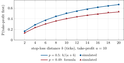
The theorem prices every take-profit and stop-loss rule on a martingale. A position whose value moves by $\pm 1$ tick with equal probability is closed at $+a$ or $-b$. The stopped value is bounded, so $\E[S_\tau] = 0$: with $\P(\text{up first}) = \pi$, $\pi a - (1 - \pi)b = 0$ and

A stop close to entry and a distant profit target win rarely and lose often, and the expected profit is zero whatever $a$ and $b$ are: the rule reshapes the distribution of the result, not its mean. With a drift ($p \ne \tfrac12$) the martingale $(q/p)^{S_n}$ gives $\pi = (1 - (q/p)^b)/(1 - (q/p)^{a+b})$; Figure 1.3 compares both formulas with simulation.

Remark 1.13 (The doubling strategy)

Doubling the stake after each loss of a fair even-money bet and stopping at the first win yields $+1$ almost surely, apparently contradicting the theorem. The stopping time is finite but unbounded, and the stopped process is not uniformly integrable: before the win it has lost $2^k - 1$ with probability $2^{-k}$. A finite credit line bounds the stakes, makes condition (ii) hold, and restores $\E[M_\tau] = 0$: a small, frequent gain paid for by a rare, enormous loss.

1.4 Changing the measure

Much of quantitative finance computes under a measure other than the one that describes the world: one under which discounted prices are martingales (chapter 5), or one under which a rare loss is common enough to simulate (chapter 26).

Definition 1.14 (Change of measure)

Two probability measures $\P$ and $\mathbb Q$ on $(\Omega, \mathcal F)$ are equivalent measures if they have the same null sets. A change of measure from $\P$ to an equivalent $\mathbb Q$ is described by the Radon–Nikodym derivative $Z = d\mathbb Q/d\P$, the almost surely unique positive random variable with $\mathbb Q(A) = \E[Z\mathbf 1_A]$ for all $A \in \mathcal F$; then $\E^{\mathbb Q}[X] = \E[ZX]$. Along a filtration, the density process is $Z_t = \E_t[Z]$, the Radon–Nikodym derivative of $\mathbb Q$ restricted to $\mathcal F_t$.

The density process is a positive $\P$-martingale with $Z_0 = 1$ (a Doob martingale), and conversely every such martingale defines a measure. Conditional expectations under the new measure follow from the old ones.

Proposition 1.15 (Bayes formula for a change of measure)

If $\mathbb Q \sim \P$ with density process $(Z_t)$ and $X$ is $\mathbb Q$-integrable, then for $s \le t$ and $X$ $\mathcal F_t$-measurable,

$$\E^{\mathbb Q}_s[X] = \frac{\E_s[Z_tX]}{Z_s}.$$

In particular, an adapted $(X_t)$ is a $\mathbb Q$-martingale if and only if $(Z_tX_t)$ is a $\P$-martingale.

Example 1.16 (Shifting a Gaussian, and seeing a far tail)

Let $X \sim \mathcal N(0, 1)$ under $\P$ and $Z = \exp(cX - c^2/2)$. Then $\E^{\mathbb Q}[e^{\iu uX}] = \E[e^{(c + \iu u)X - c^2/2}] = e^{\iu uc - u^2/2}$: under $\mathbb Q$, $X \sim \mathcal N(c, 1)$. The change of measure has moved the mean without touching the shape. Run it backwards to estimate $p = \P(X > 4) = 3.17 \times 10^{-5}$: sample $Y \sim \mathcal N(4, 1)$ and average $e^{-4Y + 8}\mathbf 1_{\{Y > 4\}}$, the indicator reweighted by $d\P/d\mathbb Q$. With 100 000 draws, plain sampling sees three exceedances and has a standard error of $1.7 \times 10^{-5}$, half the answer; the reweighted estimate has a standard error of $2.1 \times 10^{-7}$, eighty times smaller. Chapter 26 turns this into importance sampling, and chapter 5 does the same computation for whole Brownian paths.

1.5 The notation of the series

Every book of the series from this one on uses the symbols below. They extend the tables of One Quant Books 1 and 2, whose meanings are kept: $s_t$ is the bid–ask spread, $\mathcal S$ a credit spread, $\tau = T - t$ a time to expiry, $r$ a rate, $\ell$ a borrow fee, $K$ a strike, $P(t,T)$ a discount factor, $y$ a yield, $\delta$ an accrual fraction and $R$ a recovery rate. A symbol a chapter declares local may carry another meaning there.

Notation 1.17 (Probability, measures and processes)

$(\Omega,\mathcal F,\P)$, $\mathbb F = (\mathcal F_t)$	probability space; filtration (usual conditions)
$\E_t[X] = \E[X \mid \mathcal F_t]$, $\E^{\mathbb Q}_t$	conditional expectation; under another measure
$\P$, $\mathbb Q$, $B_t = e^{\int_0^t r_s\,ds}$	real-world measure; risk-neutral measure; money-market account
$\mathcal N_t$, $\mathbb Q^{\mathcal N}$; $\mathbb Q^T$, $\mathbb Q^A$	generic numeraire and its measure; $T$-forward and annuity measures
$d\mathbb Q/d\P$, $Z_t$	Radon–Nikodym derivative; density process
$\Phi$, $\varphi$; $\mathcal N(m, s^2)$	standard normal cdf and pdf (never $N(d_1)$); the normal law, always with arguments
$\varphi_X(u) = \E[e^{\iu uX}]$	characteristic function, always subscripted
$\mathbf 1_A$; $\overset{d}{=}$, $\xrightarrow{d}$, $\xrightarrow{\P}$	indicator; equality and convergence in law, in probability
$\tau$	a stopping time; where it meets a time to expiry, write $T - t$; default times are subscripted ($\tau_C$)
$W_t$; $W^{\mathbb Q}_t$	Brownian motion under the measure in force; decorated when two measures appear
$[X]_t$, $[X,Y]_t$, $\mathcal E(X)_t$	quadratic variation, covariation, stochastic exponential
$dX = \mu\,dt + \sigma\,dW$; $\mathcal L$, $\mathcal L^*$	a diffusion; its generator and the adjoint
$dX = \kappa(\bar x - X)\,dt + \sigma\,dW$	Ornstein–Uhlenbeck: speed $\kappa$, level $\bar x$, half-life $\ln 2/\kappa$
$dv = \kappa(\bar v - v)\,dt + \eta\sqrt v\,dW$	square-root process; Feller condition $2\kappa\bar v \ge \eta^2$; $\eta$ is the vol-of-vol throughout
$N_t$, $t_1 < t_2 < \dots$	counting process and its event times
$\lambda_t$, $\Lambda_t = \int_0^t\lambda_s\,ds$	intensity (Poisson rate, hazard rate, Hawkes intensity $\lambda_t = \mu + \sum_{t_i < t}g(t - t_i)$); compensator
$(\sigma^2, \nu, \gamma)$, $\psi$	Lévy triplet and characteristic exponent, $\varphi_{X_t}(u) = e^{t\psi(u)}$
$H$, $W^H_t$	Hurst exponent; fractional Brownian motion

Notation 1.18 (Statistics, matrices and numerics)

$n$, $\theta \in \Theta$, $\theta_0$	sample size, parameter, true value; hat an estimate, tilde a shrunk estimate, bar a sample mean
$\ell_n(\theta)$, $\mathcal I(\theta)$	log-likelihood (always with subscript and argument); Fisher information
$\mathrm{se}(\hat\theta)$; $\mathrm{SR}$, $\widehat{\mathrm{SR}}$	standard error; Sharpe ratio and its estimate
$R_t = \ln(S_t/S_{t-1})$	log return ($R$ alone stays the recovery rate)
$L$, $\Delta = 1 - L$; $\gamma(h)$, $\rho(h)$	lag and difference operators; autocovariance, autocorrelation
$\phi_i$, $\vartheta_j$, $\varepsilon_t$	autoregressive and moving-average coefficients (always indexed); innovations
$\mathrm{RV}_t$, $\mathrm{IV}_t$; $\sigma_{\mathrm{imp}}$	realised and integrated variance; implied volatility (never “IV” in a formula)
$\Sigma$, $C$, $\hat\Sigma$; $\mathbf 1$, $I_n$, ${}^\top$	covariance, correlation, sample covariance; ones vector, identity, transpose; vectors are columns
$\lambda_1 \ge \dots \ge \lambda_N$, $\operatorname{cond}(A)$	eigenvalues (always indexed); condition number
$\min f(x)$ s.t. $g_i(x) \le 0$, $h_j(x) = 0$	optimisation; multipliers $u \ge 0$, $v$; optimum $x^\star$, values $p^\star$, $d^\star$
$\mathrm{fl}(x)$, $u = 2^{-53}$, $\varepsilon_{\mathrm{mach}} = 2^{-52}$	floating point in binary64, round to nearest; $\mathrm{ulp}(x)$
$t_k = k\Delta t$, $x_j$, $V^k_j$; $M$, $\hat V_M$	time grid, space grid, numerical solution; Monte Carlo paths and estimator

The options, rates, credit and risk symbols ($\sigma_{\mathrm{imp}}(K,T)$, $k = \ln(K/F_{0,T})$, $\xi_t(u)$, the Greeks with the rate Greek written Rho because $\rho$ is always a correlation, $S_{a,b}(t)$, $A_{a,b}(t)$, $Q_C(t)$, $\mathrm{VaR}_{\alpha,h}$, $\mathrm{ES}_{\alpha,h}$) come from the same table and are introduced in One Quant Books 5 and 6.

1.6 Tutorial: the Doob martingale of a card game

1.7 Build: martingale diagnostics

1.8 Exercises

Exercise 1.1 ★

In the five-card game, what is the forecast of the sum after the first card turns out to be a king?

Solution

Solution of Exercise 1.1.

$M_1 = 13 + 4 \times (364 - 13)/51 = 13 + 27.53 = 40.53$, against 35 before the deal.

Exercise 1.2 ★

Which of these are stopping times for the filtration of observed prices: (a) the first time the price is 1% above the open; (b) the time of the day’s low; (c) 15:50; (d) the first time after 15:50 that the forecast of the close moves by more than 10 cents?

Solution

Solution of Exercise 1.2.

(a) Yes: whether it has happened is known at each instant. (b) No: the low is known only at the close. (c) Yes: a deterministic time is a stopping time. (d) Yes, provided the forecast is itself adapted to the observed information.

Exercise 1.3 ★

A position on a fair $\pm1$-tick walk is closed at $+1$ or $-3$. What is the probability of the take-profit, and why is the expected profit still zero?

Solution

Solution of Exercise 1.3.

$b/(a+b) = 3/4$. The stopped walk is bounded, so optional stopping gives $\E[S_\tau] = 0$: $\tfrac34 \times 1 - \tfrac14 \times 3 = 0$. Winning often is paid for by losing more when it loses.

Exercise 1.4 ★★

A forecast of the close is revised by independent news of equal variance in each of the 390 minutes of a session, and nothing else. What share of the close’s variance is resolved in the last half hour?

Solution

Solution of Exercise 1.4.

The revisions are orthogonal with equal variances, so the last 30 minutes resolve $30/390 = 7.7\%$ of the variance.

Exercise 1.5 ★★

Under $\P$, $X \sim \mathcal N(0,1)$, and $d\mathbb Q/d\P = \exp(cX - c^2/2)$. Compute $\E^{\mathbb Q}[X]$ and $\mathbb Q(X > c)$, and check that $\mathbb Q$ is a probability measure.

Solution

Solution of Exercise 1.5.

$\E[Z] = e^{-c^2/2}\E[e^{cX}] = 1$ and $Z > 0$, so $\mathbb Q$ is a probability measure equivalent to $\P$. Its characteristic function is $e^{\iu uc - u^2/2}$ (Example 1.16): $X \sim \mathcal N(c,1)$ under $\mathbb Q$, so $\E^{\mathbb Q}[X] = c$ and $\mathbb Q(X > c) = \tfrac12$.

Exercise 1.6 ★★

The under-reacting card forecaster publishes $F_k = 35 + a(M_k - 35)$ for $k \le 4$ and $F_5 = M_5$. Compute $\E[F_5 - F_4 \mid \mathcal F_4]$ and the slope of the regression of $F_5 - F_4$ on $F_4 - 35$.

Solution

Solution of Exercise 1.6.

$\E_4[F_5] = \E_4[M_5] = M_4$, so $\E[F_5 - F_4 \mid \mathcal F_4] = (1 - a)(M_4 - 35) = \frac{1 - a}{a}(F_4 - 35)$: the revision is predictable, and the slope is $(1 - a)/a = 0.667$ at $a = 0.6$. The same slope appears on the previous revision $F_4 - F_3 = a(M_4 - M_3)$, because $M_4 - 35$ is a sum of orthogonal revisions of which $M_4 - M_3$ is one.

Exercise 1.7 ★★★

Coding. With revision_regression, estimate the slope of the last revision of the under-reacting card forecaster ($a = 0.6$) on the previous revision over 20 000 seeded deals, and compare it with the answer to Exercise 1.6.

Solution

Solution of Exercise 1.7.

0.661 with a $t$-statistic of 45.9, against 0.667 in theory; the honest forecaster’s slope is $-0.005$.

Exercise 1.8 ★★★

Find the flaw. “Over a year our fair-value model’s revisions averaged zero to four decimals, so the model is a martingale and nobody can trade against it.” Correct it.

Solution

Solution of Exercise 1.8.

A mean of zero is necessary, not sufficient: the under-reacting card forecaster also has revisions averaging zero. A martingale’s revisions must be unpredictable from everything known before them, starting with its own past revisions, and the test is a regression of revisions on earlier information, with standard errors that allow for the clustering of volatility (chapter 11) and a correction for the many signals one tries (chapter 12).

1.9 Problem: The Fair Value of the Close

Problem 1.1

Weekend problem — how much of the close is still unknown at ten to four

A desk publishes $M_t = \E_t[C]$, its forecast of a stock’s closing price $C$. In its model the price starts at USD 100 and moves in each of the 390 minutes of the session by independent Gaussian increments with a total standard deviation of USD 1.80 over the day; at 15:50 the imbalance of the closing auction is published, which moves the forecast by an independent Gaussian amount $J$ with standard deviation USD 0.30 and zero mean; the last ten minutes of the session follow.

Part I — The forecast.

1. What are the variance and standard deviation of $C$?
2. Write $M_t$ before 15:50 and after the news, in terms of the observed price.
3. Why is $(M_t)$ a martingale for the desk’s filtration?
4. What is the revision of $M$ at the 15:50 news?
5. What is the probability that the news moves the forecast by more than 14 cents?

Part II — What is resolved when.

6. Why do the variances of the revisions add up to $\Var(C)$?
7. What share of $\Var(C)$ is resolved by noon?
8. What share is resolved at the news itself?
9. What share is resolved from the news to the close, inclusive?
10. Check this share against the simulation of 20 000 days.

Part III — A forecast that is too slow.

11. A second desk adds only half of $J$ at 15:50 and the other half at the close. Is its forecast a martingale?
12. What is the correlation between its 15:50 revision and its revision over the last ten minutes?
13. What slope does the regression of the second revision on the first give, in theory and in the simulation?
14. How many days of data does the test need for the slope’s $t$-statistic to reach 2?
15. A trader buys one share from that desk at its forecast at 15:50 when its revision is positive, sells one when it is negative, and closes at the close. What does it earn on average per share?

Part IV — Judgement.

16. If the last ten minutes carry three times the per-minute variance of the rest of the day (with the day’s total unchanged), what share is resolved from the news to the close?
17. Does the answer depend on the price level?
18. Why does the share matter to a trader who can only act in the closing auction?
19. State the named result: the share of the close’s variance resolved from 15:50.
20. In one sentence: what does the martingale property of a forecast promise, and what does it not?

Solution

Solution of Problem 1.1.

1. $\Var(C) = 1.80^2 + 0.30^2 = 3.33$; standard deviation USD 1.82. 2. Before the news, $M_t = S_t$, the price observed at $t$ (the remaining increments and $J$ have mean zero); after it, $M_t = S_t + J$. 3. It is the Doob martingale $\E_t[C]$ of an integrable variable. 4. $J$. 5. $\P(|J| > 0.14) = 2(1 - \Phi(0.14/0.30)) = 64.1\%$. 6. The revisions are orthogonal (Proposition 1.8), so their variances add, and $M_0$ is a constant. 7. $150/390 \times 3.24/3.33 = 37.4\%$. 8. $0.09/3.33 = 2.7\%$. 9. $(0.09 + 10/390 \times 3.24)/3.33 = 5.2\%$: 2.7% at the news and 2.5% in the last ten minutes. 10. 5.23% in the 20 000 simulated days. 11. No: its revision over the last ten minutes contains $J/2$, which its 15:50 revision $J/2$ predicts. 12. The two revisions are $J/2$ and $J/2 +$ ten minutes of increments; the correlation is $0.15^2/(0.15\sqrt{0.15^2 + 0.0831}) = 0.46$. 13. Slope $\Cov/\Var = 0.15^2/0.15^2 = 1$; the simulation gives 0.98 with a $t$-statistic of 72 over 20 000 days. 14. With $t = r\sqrt{n - 1}/\sqrt{1 - r^2}$, $t = 2$ needs $n = 4(1 - r^2)/r^2 + 1 = 16$ days. 15. The trade earns $C - (S + J/2)$ times the sign of $J$, whose mean is $\E|J|/2 = 0.5 \times 0.30\sqrt{2/\pi} = 0.120$: 12 cents a share. 16. The last ten minutes then carry $3.24 \times 30/410 = 0.237$, and the share is $(0.09 + 0.237)/3.33 = 9.8\%$. 17. No, if both standard deviations scale with the price: the shares are ratios of variances. 18. What is resolved after the last moment one can act is risk one carries, not information one can use; a trader deciding at 15:50 faces 5.2% of the day’s variance, not 100%. 19. Named result: the fair value of the close: in the model, 5.2% of the variance of the closing price is resolved from the 15:50 news to the close (2.7% by the news itself), and 9.8% if the last ten minutes are three times as volatile. 20. It promises that the revisions cannot be predicted from the forecaster’s own information, so nobody with that information can trade profitably against it; it promises nothing about accuracy.

1.10 Interview questions

Interview question 1.1 ★ trader

You play a fair coin game for a dollar a toss and stop as soon as you are one dollar up. Isn’t that a guaranteed win?

Solution

Solution of Interview question 1.1.

With unlimited time and credit you stop at $+1$ almost surely, but the stopping time is unbounded and the losses before it are not uniformly integrable; with any finite credit $b$ you win $+1$ with probability $b/(b+1)$ and lose $b$ otherwise: expected value zero.

What the interviewer is looking for: optional stopping and why its conditions matter.

Interview question 1.2 ★ researcher

What is a martingale? Is a stock price one?

Solution

Solution of Interview question 1.2.

An adapted integrable process whose conditional expectation of any future value is its current value. A stock price has a positive expected return under the real-world measure, so it is a submartingale there; discounted by the money-market account it is a martingale under the risk-neutral measure (chapter 5).

What the interviewer is looking for: the definition and the role of the measure.

Interview question 1.3 ★★ researcher, mle

Show that the increments of a martingale are uncorrelated. What does that imply for a forecast you publish?

Solution

Solution of Interview question 1.3.

For $j < k$, $\E[D_jD_k] = \E[D_j\E_{k-1}[D_k]] = 0$. A forecast that is an honest conditional expectation has revisions no one can predict from its past revisions; if a regression of today’s revision on yesterday’s has a slope, the forecast is inefficient.

What the interviewer is looking for: taking out what is known, and the testable consequence.

Interview question 1.4 ★★ trader

At the imbalance publication your forecast of the close moves 14 cents; a competitor’s moves 7 cents, then another 7 at the close, every day. What do you do?

Solution

Solution of Interview question 1.4.

The competitor’s second revision is predictable from its first, so its forecast is not a martingale: it under-reacts. Trade against its stale price at 15:50 in the direction of the news; in the chapter’s model this earns half the mean absolute news, 12 cents a share.

What the interviewer is looking for: predictable revisions mean an exploitable forecast.

Interview question 1.5 ★★ researcher, risk

When is $\E[X \mid Y]$ the linear regression of $X$ on $Y$?

Solution

Solution of Interview question 1.5.

$\E[X \mid Y]$ is the best predictor among all functions of $Y$; the linear regression is the best among affine ones. They coincide when $\E[X \mid Y]$ is affine, as it is when $(X, Y)$ is jointly Gaussian.

What the interviewer is looking for: projections onto nested subspaces; the Gaussian case.

Interview question 1.6 ★★★ developer, researcher

Design a daily check that a real-time fair-value service behaves like a martingale. What can make the check lie?

Solution

Solution of Interview question 1.6.

Store every published value with its timestamp; each day regress revisions over fixed horizons on the previous revision and on other information available at the earlier time (order-book imbalance, recent trades), with robust standard errors, and report the variance shares by time of day. It lies if horizons overlap (serially correlated errors), if the volatility is heteroskedastic and the standard errors ignore it, if the timestamps are those of publication rather than of the information (look-ahead), if many signals are tested and the best one is reported, and if the final value is itself revised.

What the interviewer is looking for: regression of revisions on prior information, and the ways the test fails.