Quantitative Methods · Methods

27Finite-Difference Methods

The morning after a grid refinement, a new pricer’s gamma near the strike shows a sawtooth. The prices have converged to the cent; their second derivative oscillates from node to node, positive, negative, positive, with swings twenty times the true gamma, and the hedger’s limits flash red for no market reason. Refining the grid again makes the sawtooth twice as large. Nothing is wrong with the equation or the code in the ordinary sense: the time-stepping scheme is doing exactly what its amplification factor says it will. This chapter discretises the backward equations of chapter 4 on a grid, analyses consistency, stability and oscillations, and builds the solver the firm uses for one- and two-factor problems.

27.1 Discretising a parabolic equation

By the Feynman–Kac formula, a European price $u(\tau, x)$ in time to maturity $\tau$ and log-price $x = \ln S$ solves $u_\tau = \mathcal Lu$ with $\mathcal Lu = au_{xx} + bu_x - cu$ , $a = \frac12\sigma^2$ , $b = r - \frac12\sigma^2$ , $c = r$ , from the payoff at $\tau = 0$ .

Definition 27.1 (Finite-difference method, method of lines, non-uniform grid)

A finite-difference method replaces the derivatives of a differential equation by difference quotients of the values on a grid of nodes. The method of lines discretises space first, turning the equation into a system of ordinary differential equations $\dot U = L_hU$ in time, then applies a time-stepping scheme. On a non-uniform grid the spacings $h_i^- = x_i - x_{i-1}$ and $h_i^+ = x_{i+1} - x_i$ differ; the three-point formulas

u_{xx} \approx \frac{2u_{i-1}}{h^-(h^- + h^+)} - \frac{2u_i}{h^-h^+} + \frac{2u_{i+1}}{h^+(h^- + h^+)},

u_x \approx \frac{-h^+u_{i-1}}{h^-(h^- + h^+)} + \frac{(h^+ - h^-)u_i}{h^-h^+} + \frac{h^-u_{i+1}}{h^+(h^- + h^+)}

are exact on quadratics.

Definition 27.2 (Truncation error, consistent and stable schemes)

The truncation error of a scheme is the residual left when the exact solution is substituted into it. A scheme is a consistent scheme if its truncation error tends to zero with the steps, and a stable scheme if its solutions stay bounded, uniformly in the steps, over a fixed time interval.

Theorem 27.3 (Lax equivalence theorem)

For a well-posed linear initial-value problem, a consistent finite-difference scheme converges if and only if it is stable (Lax and Richtmyer, 1956).

The theorem divides the work: consistency is Taylor’s theorem, and stability is the subject of the next two sections. The firm’s operator (Section 27.6) builds the tridiagonal $L_h$ on any grid; each implicit step is one solve by the tridiagonal matrix algorithm of chapter 25, $O(n)$ operations. A grid stretched by $x_i = x^* + \alpha\sinh(\xi_i)$ with uniform $\xi_i$ puts nodes where the payoff bends: with $\alpha = 0.05$ around the strike, it cuts the call’s price error by a factor of about 2.9 at equal node count (0.0079 against 0.0225 with 50 nodes, 0.00012 against 0.00035 with 400).

27.2 Explicit, implicit and theta schemes

Definition 27.4 (Explicit, implicit, theta and Crank–Nicolson schemes)

With time step $\Delta\tau$ , the theta scheme is $(I - \theta\Delta\tau L_h)U^{n+1} = (I + (1 - \theta)\Delta\tau L_h)U^n$ . It is the explicit scheme (forward Euler) for $\theta = 0$ , the implicit scheme (backward Euler) for $\theta = 1$ and the Crank–Nicolson scheme (Crank and Nicolson, 1947) for $\theta = \frac12$ ; its time error is $O(\Delta\tau)$ except at $\theta = \frac12$ , where it is $O(\Delta\tau^2)$ .

Definition 27.5 (Von Neumann stability analysis, CFL condition)

Von Neumann stability analysis substitutes a Fourier mode $U_j^n = g^ne^{\mathrm ij\xi}$ into a constant-coefficient scheme and requires $|g(\xi)| \le 1 + O(\Delta\tau)$ for every frequency. The CFL condition (Courant, Friedrichs and Lewy, 1928) is the resulting restriction of the time step by the space step for an explicit scheme.

Proposition 27.6 (Amplification factors of the theta schemes)

For $u_\tau = au_{xx}$ on a uniform grid, with $\lambda = a\Delta\tau/\Delta x^2$ and $s = \sin^2(\xi/2)$ ,

g(\xi) = \frac{1 - 4(1 - \theta)\lambda s}{1 + 4\theta\lambda s}.

The explicit scheme is stable if and only if $\lambda \le \frac12$ , that is $\Delta\tau \le \Delta x^2/\sigma^2$ ; the implicit and Crank–Nicolson schemes are stable for every $\lambda$ .

Proof. $U_{j+1} - 2U_j + U_{j-1} = (e^{\mathrm i\xi} - 2 + e^{-\mathrm i\xi})U_j = -4sU_j$ , and substituting into the scheme gives $g$ . At $\xi = \pi$ the explicit factor is $1 - 4\lambda$ , which is at least $-1$ iff $\lambda \le \frac12$ . For $\theta \ge \frac12$ the numerator is at least $-1$ times the denominator for every $\lambda$ , so $|g| \le 1$ . ∎

The limit is sharp. With 200 nodes over the grid, the explicit scheme at $\lambda = 0.489$ (409 steps) prices the three-month call at 4.3576 against Black–Scholes 4.3576; at $\lambda = 0.509$ (393 steps) the highest frequency is multiplied by $-1.04$ at each step, and the largest value on the grid is 2 413.

27.3 Stability and oscillations

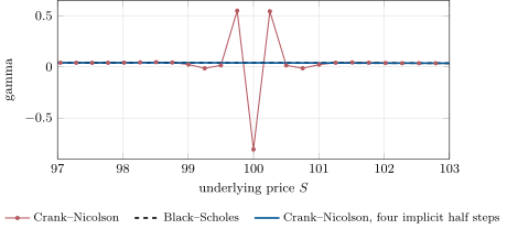
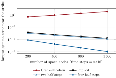
Stability in the sense of the Lax theorem is not enough for Greeks. At the highest frequency, the Crank–Nicolson factor is $(1 - 2\lambda)/(1 + 2\lambda)$ : bounded by one, but close to $-1$ when $\lambda$ is large (Figure 27.1). A kinked payoff contains every frequency, and Crank–Nicolson damps its highest ones by almost nothing while flipping their sign at every step. With 400 nodes and 25 steps for a three-month call ( $\lambda = 32$ ), the price at the strike is within 0.018 of Black–Scholes, and the gamma oscillates between $-0.81$ and $0.55$ around a true value of 0.040 (Figure 27.2). Refining space and time together doubles $\lambda$ and the sawtooth: the largest gamma error is 0.46, 0.84, 1.69 and 3.38 on 200, 400, 800 and 1 600 nodes. That is the morning after the refinement.

Von Neumann amplification factors of the theta schemes for u_ = au_xx against the frequency. The explicit scheme leaves [-1, 1] just above = 1/2; at = 32 the implicit scheme kills the high frequencies and Crank–Nicolson flips their sign with almost no damping. Data: the chapter’s tutorial. — **Figure 27.1.** Von Neumann amplification factors of the theta schemes for $u_\tau = au_{xx}$ against the frequency. The explicit scheme leaves $[-1, 1]$ just above $\lambda = \frac12$ ; at $\lambda = 32$ the implicit scheme kills the high frequencies and Crank–Nicolson flips their sign with almost no damping. Data: the chapter’s tutorial.

Gamma of a three-month at-the-money call from Crank–Nicolson on 400 log-price nodes and 25 time steps (= 32), with and without Rannacher start-up, near the strike (the markers are the grid nodes); the last curve lies on the Black–Scholes gamma. Data: the chapter’s tutorial. — **Figure 27.2.** Gamma of a three-month at-the-money call from Crank–Nicolson on 400 log-price nodes and 25 time steps ( $\lambda = 32$ ), with and without Rannacher start-up, near the strike (the markers are the grid nodes); the last curve lies on the Black–Scholes gamma. Data: the chapter’s tutorial.

Definition 27.7 (Rannacher time-stepping)

Rannacher time-stepping (Rannacher, 1984) replaces the first Crank–Nicolson steps by implicit Euler steps of half the size, which damp the high frequencies of non-smooth initial data, and continues with Crank–Nicolson.

Two implicit half steps remove the sawtooth (gamma error $4.7 \times 10^{-4}$ at 400 nodes) but leave a first-order error, halving with each refinement; four restore second order, the error falling by 4.05 and 4.07 per halving ( $1.76 \times 10^{-5}$ , $4.35 \times 10^{-6}$ , $1.07 \times 10^{-6}$ ; Figure 27.3). The price tells the same story more quietly: plain Crank–Nicolson converges only at first order on this problem (errors 0.041, 0.018, 0.0092, 0.0046), with the start-up at second order. Giles and Carter (2006) analyse the mechanism.

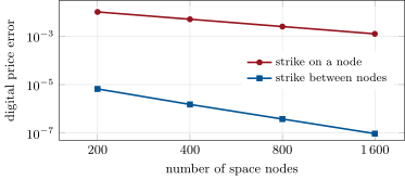
Largest gamma error of the three-month call for 90 < S < 110 as space and time are refined together: plain Crank–Nicolson diverges, the implicit scheme and Crank–Nicolson with two implicit half steps converge at first order, and with four at second order. Data: the chapter’s tutorial. — **Figure 27.3.** Largest gamma error of the three-month call for $90 < S < 110$ as space and time are refined together: plain Crank–Nicolson diverges, the implicit scheme and Crank–Nicolson with two implicit half steps converge at first order, and with four at second order. Data: the chapter’s tutorial.

The payoff’s placement on the grid matters as much. A digital paying 1 above the strike, with the strike on a node (where the payoff is set to $\frac12$ ), converges at first order even with the start-up (error $9.9 \times 10^{-3}$ on 200 nodes, halving each time) and does not converge at all without it (about 0.1 at every level). With the strike midway between two nodes, which is the same as averaging the payoff over each node’s cell, the error is $6.6 \times 10^{-6}$ on 200 nodes and falls by 4 per halving (Figure 27.4). Pooley, Vetzal and Forsyth (2003) report the same pattern: averaging the initial data or shifting the grid is not sufficient alone, and restores the expected convergence when combined with a smoothing start.

**Figure 27.4.** Price error of a three-month digital at the strike, Crank–Nicolson with four implicit half steps: the strike on a node gives first order, the strike midway between nodes second order. Data: the chapter’s tutorial.

27.4 Boundaries, monotonicity and extrapolation

Definition 27.8 (M-matrix, upwind scheme)

An M-matrix is a real square matrix with nonpositive off-diagonal entries whose inverse exists and is entrywise nonnegative. An upwind scheme discretises the first derivative by the one-sided difference taken towards the direction the drift comes from, where the central difference would make an off-diagonal coefficient of $L_h$ negative.

Proposition 27.9 (Monotone schemes)

If the off-diagonal entries of $L_h$ are nonnegative and $c \ge 0$ , the implicit step matrix $I - \Delta\tau L_h$ is an M-matrix for every $\Delta\tau$ , so the implicit scheme maps nonnegative data to nonnegative solutions and preserves order: a larger payoff gives a larger price, and no new extremum appears.

Proof. The off-diagonal entries of $I - \Delta\tau L_h$ are nonpositive and each row’s diagonal exceeds the sum of the magnitudes of its off-diagonal entries (the rows of $L_h$ sum to $-c \le 0$ ), so the matrix is strictly diagonally dominant with a positive diagonal: an M-matrix, with a nonnegative inverse. ∎

Central differences keep the sign pattern while $|b|\Delta x \le 2a$ . For a low-volatility, high-rate digital ( $\sigma = 2\%$ , $r = 5\%$ , $\Delta x = 0.02$ ) the ratio $b\Delta x/(2a)$ is 2.49; the implicit scheme with central differences then returns a digital worth 1.030 somewhere on the grid, more than the discounted payout of 0.951, and a price that is not monotone in $S$ (total variation 1.23); upwinding returns 0.951 and a monotone profile, at the price of first-order accuracy in the drift term. At the far ends of the grid the solver imposes either known values (a Dirichlet condition such as $u = S - Ke^{-r\tau}$ for a deep in-the-money call) or zero gamma, extrapolating linearly; with the grid at five standard deviations the two give prices at the strike that differ by $6 \times 10^{-8}$ .

Definition 27.10 (Richardson extrapolation)

Richardson extrapolation (Richardson, 1911) combines two approximations $u_h$ and $u_{h/2}$ whose error is $Ch^p$ into $u_{h/2} + (u_{h/2} - u_h)/(2^p - 1)$ , which cancels the leading term.

It works only if the order is what it is assumed to be: with the start-up, the call’s price errors on 200 and 400 nodes are $1.8 \times 10^{-3}$ and $4.6 \times 10^{-4}$ , and the extrapolated value with $p = 2$ is within $3.2 \times 10^{-7}$ . Applied to plain Crank–Nicolson, whose error is first order here, it would remove the wrong term.

27.5 Alternating directions

Definition 27.11 (Alternating direction implicit method)

An alternating direction implicit method (Peaceman and Rachford, 1955; Douglas and Rachford, 1956) splits a multi-dimensional operator $L = A_0 + A_1 + A_2$ , with $A_1$ and $A_2$ acting along one coordinate each and $A_0$ the mixed-derivative part, and treats one direction implicitly at a time. The Douglas scheme is $Y_0 = U^n + \Delta\tau LU^n$ , $Y_j = Y_{j-1} + \theta\Delta\tau A_j(Y_j - U^n)$ for $j = 1, 2$ , $U^{n+1} = Y_2$ .

Each stage solves one tridiagonal system per grid line, so a step costs $O(n^2)$ on an $n \times n$ grid instead of a two-dimensional solve. The mixed derivative is explicit, which is what makes the stability of the scheme delicate: conditions on $\theta$ for unconditional stability with mixed-derivative terms were analysed by Craig and Sneyd (1988) and by in ’t Hout and Welfert (2007), and in ’t Hout and Foulon (2010) compare the Douglas, Craig–Sneyd and Hundsdorfer–Verwer schemes on the Heston equation (stated, not proved here); the firm uses $\theta = \frac12$ . On an exchange option $\max(S_1 - S_2, 0)$ with $\sigma_1 = 30\%$ , $\sigma_2 = 20\%$ and correlation 0.5, whose price is 10.5243 by Margrabe’s formula, the firm’s solver errs by 0.045, 0.026 and 0.014 on grids of $40^2$ , $80^2$ and $160^2$ nodes: first order, because the payoff’s kink runs along the diagonal between nodes, which the digital above has already shown to be the usual culprit.

27.6 Tutorial: the sawtooth gamma

Goal. Price a three-month call on a log-price grid with the three schemes, see the explicit limit, the Crank–Nicolson sawtooth and its removal. End state: Figures 27.2 and 27.3 and the convergence ratios.

The operator. Three-point coefficients on any grid, with optional upwinding.

def operator(x: np.ndarray, a, b, c, upwind: bool = False) -> tuple:
    """Coefficients of L u = a u_xx + b u_x - c u at interior nodes 1..n-1 on a (possibly non-uniform) grid:
    (L u)_i = lo_i u_{i-1} + di_i u_i + up_i u_{i+1}. Central first differences are second order; `upwind` uses the
    one-sided difference in the direction of the drift where the central one would break the M-matrix sign pattern."""
    xi = x[1:-1]
    hm, hp = xi - x[:-2], x[2:] - xi
    av = np.broadcast_to(np.asarray(a(xi) if callable(a) else a, dtype=float), xi.shape)
    bv = np.broadcast_to(np.asarray(b(xi) if callable(b) else b, dtype=float), xi.shape)
    cv = np.broadcast_to(np.asarray(c(xi) if callable(c) else c, dtype=float), xi.shape)
    lo = 2 * av / (hm * (hm + hp))
    up = 2 * av / (hp * (hm + hp))
    di = -lo - up - cv
    central_lo, central_up = -bv * hp / (hm * (hm + hp)), bv * hm / (hp * (hm + hp))
    central_di = bv * (hp - hm) / (hm * hp)
    if upwind:
        bad = (lo + central_lo < 0) | (up + central_up < 0)
        fwd = bad & (bv > 0)
        bwd = bad & (bv < 0)
        central_lo = np.where(fwd, 0.0, np.where(bwd, -bv / hm, central_lo))
        central_up = np.where(fwd, bv / hp, np.where(bwd, 0.0, central_up))
        central_di = np.where(fwd, -bv / hp, np.where(bwd, bv / hm, central_di))
    return lo + central_lo, di + central_di, up + central_up

Listing 27.1. The operator

au_{xx} + bu_x - cu

on a non-uniform grid (Python). code/firm/pde/firm_pde.py

The time step and the start-up, in the C++20 twin (the Rust twin is line for line the same).

// one theta step (I - theta dt L) u' = (I + (1 - theta) dt L) u with linear extrapolation at both ends
inline std::vector<double> theta_step(const std::vector<double>& x, const std::vector<double>& u, const Tridiag& L,
                                      double dt, double theta) {
    const std::size_t m = x.size() - 2;
    std::vector<double> rhs(m), alo(m), adi(m), aup(m);
    for (std::size_t k = 0; k < m; ++k) {
        rhs[k] = u[k + 1] + (1 - theta) * dt * (L.lo[k] * u[k] + L.di[k] * u[k + 1] + L.up[k] * u[k + 2]);
        alo[k] = -theta * dt * L.lo[k];
        adi[k] = 1 - theta * dt * L.di[k];
        aup[k] = -theta * dt * L.up[k];
    }
    const std::size_t n = x.size() - 1;
    const double l0 = x[1] - x[0], l1 = x[2] - x[1], r0 = x[n] - x[n - 1], r1 = x[n - 1] - x[n - 2];
    adi[0] += alo[0] * (1 + l0 / l1);
    aup[0] += alo[0] * (-l0 / l1);
    adi[m - 1] += aup[m - 1] * (1 + r0 / r1);
    alo[m - 1] += aup[m - 1] * (-r0 / r1);
    const auto inner = thomas(alo, adi, aup, rhs);
    std::vector<double> out(n + 1);
    for (std::size_t k = 0; k < m; ++k) out[k + 1] = inner[k];
    out[0] = out[1] - (out[2] - out[1]) * l0 / l1;
    out[n] = out[n - 1] + (out[n - 1] - out[n - 2]) * r0 / r1;
    return out;
}

// march from the payoff to tau: `rannacher` implicit half steps replace the first rannacher / 2 steps
inline std::vector<double> solve_1d(const std::vector<double>& x, std::vector<double> u, double a, double b, double c,
                                    double tau, int n_steps, double theta, int rannacher) {
    const Tridiag L = operator_1d(x, a, b, c);
    const double dt = tau / n_steps;
    for (int k = 0; k < rannacher; ++k) u = theta_step(x, u, L, dt / 2, 1.0);
    for (int k = 0; k < n_steps - rannacher / 2; ++k) u = theta_step(x, u, L, dt, theta);
    return u;
}

Listing 27.2. Theta step with linear boundaries, and Rannacher start-up (C++20). code/firm/pde/cpp/firm_pde.hpp

Run explicit_blowup(), sawtooth(), convergence(), digital_placement(), stretched(), richardson_demo(), upwind_demo() and adi_exchange() in qm_fd.py; then fig_fd.py.

What to change next. Price a down-and-out call with the barrier on a node and between nodes; add Rannacher start-up at each discrete monitoring date; try $\theta = 0.51$ instead of the start-up.

27.7 Build: the finite-difference solver

Purpose. One- and two-factor backward equations for the firm’s pricers, with Greeks that can be hedged on.

Interface. uniform_grid, sinh_grid; operator(x, a, b, c, upwind); solve_1d(x, payoff, a, b, c, tau, n_steps, theta, rannacher, left, right, upwind); thomas; richardson; amplification; interp; douglas_adi_2d. C++20 and Rust twins of operator_1d, thomas, theta_step and solve_1d.

Rules. Crank–Nicolson never starts on non-smooth data without implicit half steps; strikes and barriers sit midway between nodes (or the payoff is cell-averaged); the order is measured before extrapolating; a sign-pattern check flags a lost M-matrix.

Acceptance tests. code/firm/pde/{tests,cpp,rust}: Thomas against a dense solve; the operator exact on quadratics; first and second order measured; the stretched grid beats the uniform one; Dirichlet boundary; amplification factors against the direct formula; upwinding restores the sign pattern; ADI against Margrabe; C++20 and Rust against the Python values to $10^{-11}$ .

Stretch. Barriers and American exercise (the penalty method for the variational inequality of chapter 10); the Craig–Sneyd and Hundsdorfer–Verwer ADI variants; adaptive grids.

Sources and further reading

J. Crank and P. Nicolson, Proceedings of the Cambridge Philosophical Society 43, 1947; R. Courant, K. Friedrichs and H. Lewy, Mathematische Annalen 100, 1928.
P. D. Lax and R. D. Richtmyer, “Survey of the stability of linear finite difference equations”, Communications on Pure and Applied Mathematics 9, 1956.
R. Rannacher, Numerische Mathematik 43, 1984; M. B. Giles and R. Carter, Journal of Computational Finance 9(4), 2006; D. M. Pooley, K. R. Vetzal and P. A. Forsyth, “Convergence remedies for non-smooth payoffs in option pricing”, Journal of Computational Finance 6(4), 2003.
D. W. Peaceman and H. H. Rachford, Journal of SIAM 3, 1955; J. Douglas and H. H. Rachford, Transactions of the AMS 82, 1956; I. J. D. Craig and A. D. Sneyd, Computers and Mathematics with Applications 16, 1988; K. J. in ’t Hout and B. D. Welfert, Applied Numerical Mathematics 57, 2007; K. J. in ’t Hout and S. Foulon, International Journal of Numerical Analysis and Modeling 7, 2010.
L. F. Richardson, Philosophical Transactions of the Royal Society A 210, 1911.

27.8 Exercises

Exercise 27.1 ★

With $\sigma = 20\%$ and $\Delta x = 0.0025$ in log-price, what is the largest stable explicit time step, and how many steps does a one-year option need?

Solution

Solution of Exercise 27.1.

$\Delta\tau \le \Delta x^2/\sigma^2 = 6.25 \times 10^{-6}/0.04 = 1.5625 \times 10^{-4}$ years, so 6 400 steps for one year.

Exercise 27.2 ★

Two prices on grids $h$ and $h/2$ are 4.3558 and 4.3572 and the scheme is second order. What is the extrapolated price?

Solution

Solution of Exercise 27.2.

$4.3572 + (4.3572 - 4.3558)/3 = 4.35767$ .

Exercise 27.3 ★

Show that the three-point second difference on a uniform grid has truncation error $\frac{h^2}{12}u_{xxxx} + O(h^4)$ .

Solution

Solution of Exercise 27.3.

$u(x \pm h) = u \pm hu_x + \frac{h^2}{2}u_{xx} \pm \frac{h^3}{6}u_{xxx} + \frac{h^4}{24}u_{xxxx} + O(h^5)$ ; adding, subtracting $2u$ and dividing by $h^2$ leaves $u_{xx} + \frac{h^2}{12}u_{xxxx} + O(h^4)$ .

Exercise 27.4 ★★

Compute the Crank–Nicolson factor at $\xi = \pi$ for $\lambda = 32$ and the number of steps needed to damp that mode by a factor of 100. Compare with one implicit half step.

Solution

Solution of Exercise 27.4.

$g(\pi) = (1 - 64)/(1 + 64) = -0.969$ ; $|g|^n = 0.01$ needs $n = \ln100/(-\ln0.969) \approx 148$ steps, far more than the 25 of the whole run. One implicit half step at $\lambda/2 = 16$ has factor $1/(1 + 64) = 0.015$ at $\xi = \pi$ : a single half step damps that mode by 65.

Exercise 27.5 ★★

For $au_{xx} + bu_x$ with central differences on a uniform grid, find the condition on $\Delta x$ that keeps both off-diagonal coefficients nonnegative.

Solution

Solution of Exercise 27.5.

The coefficients are $a/h^2 \mp b/(2h)$ ; both are nonnegative iff $h \le 2a/|b|$ , i.e. $|b|h/(2a) \le 1$ .

Exercise 27.6 ★★

Why does a Dirichlet condition $u = 0$ at the lower end of a call’s grid barely matter, while the same condition at the upper end would ruin the price?

Solution

Solution of Exercise 27.6.

Far below the strike the call is worth almost exactly zero, so $u = 0$ is nearly the true value and its small error is damped by diffusion before it reaches the strike. Far above, the call is worth about $S - Ke^{-r\tau}$ , a large number: imposing zero there is a large error that diffuses inward and, over the option’s life, reaches the strike.

Exercise 27.7 ★★★

Coding. Price the three-month digital with the strike on a node and midway between nodes, Crank–Nicolson with four half steps, on 200 to 1 600 nodes, and give the convergence ratios.

Solution

Solution of Exercise 27.7.

digital_placement(): on a node $9.9 \times 10^{-3}$ , $4.9 \times 10^{-3}$ , $2.5 \times 10^{-3}$ , $1.2 \times 10^{-3}$ (ratios 2.0, first order); between nodes $6.6 \times 10^{-6}$ , $1.5 \times 10^{-6}$ , $3.8 \times 10^{-7}$ , $9.5 \times 10^{-8}$ (ratios 4.4, 4.0, 4.0, second order).

Exercise 27.8 ★★★

Find the flaw. “The price converged to the cent when we halved the grid, so the Greeks we compute by differencing it are right.”

Solution

Solution of Exercise 27.8.

A converged price says nothing about its derivatives: a node-to-node oscillation of size $\epsilon$ in the values becomes $\epsilon/h$ in delta and $\epsilon/h^2$ in gamma. In the chapter’s run the price is within 0.018 and the gamma wrong by twenty times its size. Greeks need their own convergence test.

27.9 Problem: The Sawtooth Gamma

Problem 27.1

Weekend problem — a Greek that gets worse with refinement

A three-month at-the-money call ( $K = 100$ , $r = 3\%$ , $\sigma = 20\%$ ) is priced by Crank–Nicolson on a log-price grid of $\pm5$ standard deviations with 400 nodes and 25 time steps.

Part I — The schemes.

What is $\lambda$ , and would the explicit scheme be stable?
Where exactly does the explicit scheme become unstable, and what happens just beyond?
What is the Crank–Nicolson amplification factor of the highest frequency at this $\lambda$ ?
How accurate is the price at the strike, and how accurate is the gamma?
What happens to the gamma error when space and time are refined together?

Part II — The remedy.

What do two implicit half steps give, and at what order?
What do four give, and at what order?
What order does plain Crank–Nicolson achieve on the price?
Why does the digital converge only at first order with the strike on a node?
What does moving the strike between nodes give?

Part III — Grids and extrapolation.

How much does the sinh grid gain at equal node count?
What does Richardson extrapolation give with the start-up, and why not without?
When do central differences lose the M-matrix property, and what does it cost here?
How do the two boundary conditions compare?
How does Douglas ADI do on the exchange option, and why only first order?

Part IV — Judgement.

What test would have caught the sawtooth before the hedgers did?
Why is a stable scheme not enough for Greeks?
What rules should the firm’s pricer enforce by default?
State the named result: the number of implicit half steps that removes the oscillation and the order it restores, from the error ratio per halving.
In one sentence: what does the amplification factor tell a quant that the price does not?

Solution

Solution of Problem 27.1.

1. $\lambda = a\Delta\tau/\Delta x^2 = 0.02 \times 0.01/0.0025^2 = 32$ ; the explicit scheme needs $\lambda \le \frac12$ . 2. At $\lambda = \frac12$ : at 0.489 (409 steps on 200 nodes) the price is 4.3576; at 0.509 (393 steps) the largest value on the grid is 2 413. 3. $(1 - 2\lambda)/(1 + 2\lambda) = -63/65 = -0.969$ . 4. The price is within 0.018 of 4.3576; the gamma swings between $-0.81$ and $0.55$ around 0.040 (largest error 0.84). 5. It doubles: 0.46, 0.84, 1.69 and 3.38 on 200 to 1 600 nodes, because $\lambda$ doubles. 6. Largest gamma error $4.7 \times 10^{-4}$ at 400 nodes, halving with each refinement: first order. 7. $1.76 \times 10^{-5}$ , $4.35 \times 10^{-6}$ , $1.07 \times 10^{-6}$ : ratios 4.05 and 4.07, second order. 8. First order: 0.041, 0.018, 0.0092, 0.0046. 9. A discontinuity sampled at a node (value $\frac12$ there) leaves an error at the strike proportional to the space step, as the measured ratios of 2 show; the loss comes from how the discontinuous data are sampled, not from the time stepping, since smaller time steps do not change it. 10. Error $6.6 \times 10^{-6}$ on 200 nodes, falling by 4 per halving. 11. About 2.9 times smaller error at equal node count (0.0079 against 0.0225 on 50 nodes). 12. From $1.8 \times 10^{-3}$ and $4.6 \times 10^{-4}$ to $3.2 \times 10^{-7}$ . Without the start-up the price error is first order, and extrapolating with $p = 2$ removes the wrong term. 13. When $|b|\Delta x/(2a) > 1$ ; here 2.49, and the digital reaches 1.030 (above the discounted payout 0.951) with total variation 1.23; upwinding restores 0.951 and monotonicity. 14. Zero gamma and Dirichlet ends give prices at the strike that differ by $6 \times 10^{-8}$ with the grid at five standard deviations. 15. Errors 0.045, 0.026 and 0.014 against Margrabe’s 10.5243 on $40^2$ , $80^2$ , $160^2$ nodes: first order, from the kink along the diagonal between nodes. 16. A refinement test on the Greeks (gamma should change by a factor 4 less per halving, not grow), or a count of sign changes of the second difference near the strike. 17. Stability bounds the growth of every mode but not its sign: Crank–Nicolson keeps high frequencies alive with alternating sign, and differencing twice amplifies them by $1/h^2$ . 18. Implicit start-up on every non-smooth datum, strikes and barriers between nodes, measured convergence orders for prices and Greeks, an M-matrix check, and extrapolation only at a measured order. 19. Named result: the sawtooth gamma: four implicit half steps remove the oscillation and restore second order, the gamma error falling by 4.05 and 4.07 per halving, where plain Crank–Nicolson’s doubles and two half steps give first order. 20. What the scheme does to each frequency at each step, which is what the Greeks see.

27.10 Interview questions

Interview question 27.1 ★ researcher, developer

What is the stability condition of the explicit scheme for the heat equation, and why does it matter for a fine grid?

Solution

Solution of Interview question 27.1.

$\Delta t \le \Delta x^2/(2a)$ for $u_t = au_{xx}$ ( $\Delta t \le \Delta x^2/\sigma^2$ in log-price). Halving $\Delta x$ quarters the time step, so a fine grid makes the explicit scheme very expensive; hence implicit schemes.

What the interviewer is looking for: The $\Delta x^2$ scaling and its cost.

Interview question 27.2 ★★ researcher

Crank–Nicolson is unconditionally stable and second order. Why does it produce oscillating Greeks, and how do you fix it?

Solution

Solution of Interview question 27.2.

Its amplification factor tends to $-1$ at high frequencies when $\Delta t/\Delta x^2$ is large, so the high-frequency content of a kinked payoff survives with alternating sign and shows up in the second difference. Fix: a few implicit (half) steps at the start (Rannacher), payoff smoothing or placement, or an L-stable scheme.

What the interviewer is looking for: The amplification factor near $-1$ and the Rannacher start.

Interview question 27.3 ★★ researcher

Where do you put the strike and the barrier relative to the grid, and why?

Solution

Solution of Interview question 27.3.

Midway between nodes (or with the payoff averaged over each cell) for strikes; exactly on a node for a continuously monitored barrier, where the boundary condition is imposed. The error of a discontinuity inside a cell depends on its position in the cell and destroys the convergence order.

What the interviewer is looking for: Placement determines the order.

Interview question 27.4 ★★ developer

How do you solve an implicit step efficiently in one dimension and in two?

Solution

Solution of Interview question 27.4.

In one dimension, the tridiagonal system is solved by the Thomas algorithm in $O(n)$ . In two, an ADI splitting solves one tridiagonal system per grid line and per direction, $O(n^2)$ per step, instead of a sparse solve of the full system.

What the interviewer is looking for: Thomas and ADI.

Interview question 27.5 ★★ researcher, risk

How would you verify that a finite-difference pricer converges at the order it claims?

Solution

Solution of Interview question 27.5.

Refine space and time together by factors of two on a problem with a known answer (or against a much finer reference), and check that the error ratio tends to $2^p$ for prices and Greeks separately, at points that stay on the grid.

What the interviewer is looking for: Error ratios per halving, including Greeks.

Interview question 27.6 ★★★ researcher

Your two-factor solver gives prices that are occasionally negative for a deep out-of-the-money digital. What is happening?

Solution

Solution of Interview question 27.6.

The scheme is not monotone: central first differences with a large drift relative to diffusion (or a mixed-derivative stencil with strong correlation) give negative off-diagonal coefficients, and Crank–Nicolson does not damp the resulting oscillations. Upwind, refine where the drift dominates, use a positivity-preserving mixed-derivative stencil, and start with implicit steps.

What the interviewer is looking for: Loss of the M-matrix property.

Terms defined in this chapter

See all 2333 terms in the glossary