Quantitative Methods · Methods

5Girsanov and Changes of Numeraire

A risk system prices a five-year caplet by simulating the short rate week by week, integrating it into a discount factor, and averaging over paths: 260 random numbers per path and a standard error of 0.05 basis point after 20 000 paths. A colleague prices the same caplet by changing the measure to the one attached to the zero-coupon bond maturing at the fixing date: under it the short rate at that date is a single Gaussian with a known mean, so each path costs one random number, and the same argument yields a closed form that takes a microsecond. The answers agree within their standard errors: 3.26 basis points of notional. Nothing about the market changed; only the unit in which values were counted. This chapter proves Girsanov’s theorem, which says what a change of measure does to a Brownian motion, defines numeraires and the martingale measures attached to them, and derives the forward and annuity measures that every rates and options chapter of the series computes with.

5.1 Girsanov’s theorem

Definition 5.1 (Novikov’s condition)

An adapted process $\gamma$ satisfies Novikov’s condition on $[0, T]$ if $\E[\exp(\tfrac12\int_0^T\gamma_s^2\,ds)] < \infty$ .

It is a sufficient condition for the positive local martingale $Z_t = \mathcal E(\int\gamma\,dW)_t = \exp(\int_0^t\gamma_s\,dW_s - \tfrac12\int_0^t\gamma_s^2\,ds)$ of Definition 3.11 to be a true martingale, with $\E[Z_T] = 1$ , so that it can serve as a density process (Definition 1.14). Bounded $\gamma$ always qualifies.

Theorem 5.2 (Girsanov)

Let $\gamma$ satisfy Novikov’s condition and define $\mathbb Q$ on $\mathcal F_T$ by $d\mathbb Q/d\P = Z_T$ . Then

W^{\mathbb Q}_t = W_t - \int_0^t\gamma_s\,ds

is a Brownian motion under $\mathbb Q$ . Conversely, every $\mathbb Q \sim \P$ on the filtration of $W$ has a density of this form.

Proof. By Theorem 3.12 it suffices that $W^{\mathbb Q}$ be a continuous $\mathbb Q$ -local martingale with $[W^{\mathbb Q}]_t = t$ ; the quadratic variation is that of $W$ , since the drift has finite variation. By Proposition 1.15, $W^{\mathbb Q}$ is a $\mathbb Q$ -local martingale if $ZW^{\mathbb Q}$ is a $\P$ -local martingale, and by the product rule, with $dZ = Z\gamma\,dW$ , $d(ZW^{\mathbb Q}) = Z\,dW^{\mathbb Q} + W^{\mathbb Q}\,dZ + d[Z, W^{\mathbb Q}] = Z\,dW - Z\gamma\,dt + W^{\mathbb Q}\,dZ + Z\gamma\,dt$ , a stochastic integral. The converse is the martingale representation theorem applied to the density process (Theorem 3.13). ∎

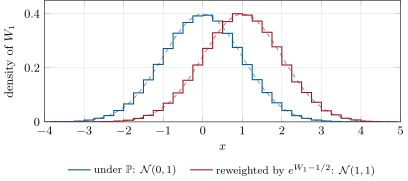
A change of measure cannot change volatility, which is visible in the quadratic variation of a single path; it changes drift, which is not. With constant $\gamma$ the theorem is the Cameron–Martin formula: reweighting paths by $e^{\gamma W_T - \gamma^2T/2}$ turns a Brownian motion into one with drift $\gamma$ (Figure 5.1). Read backwards, it removes a drift, which is how the first-passage probability with drift of chapter 2 is derived (Exercise 5.7).

The same 200 000 draws of W_1, counted plainly (blue) and weighted by the density Z_1 = e W_1 - 2/2 with = 1 (red): the weighted histogram is the N(1, 1) density (dashed), and the shape is untouched. Data: the chapter’s tutorial, seeded. — **Figure 5.1.** The same 200 000 draws of $W_1$ , counted plainly (blue) and weighted by the density $Z_1 = e^{\gamma W_1 - \gamma^2/2}$ with $\gamma = 1$ (red): the weighted histogram is the $\mathcal N(1, 1)$ density (dashed), and the shape is untouched. Data: the chapter’s tutorial, seeded.

5.2 Numeraires and their martingale measures

Definition 5.3 (Numeraire, money-market account)

A numeraire $\mathcal N$ is the price process of a traded asset (or self-financing portfolio) that is strictly positive at all times; values expressed in units of it are $V_t/\mathcal N_t$ . The money-market account is the numeraire $B_t = \exp\int_0^tr_s\,ds$ that rolls overnight at the short rate $r_t$ .

Definition 5.4 (Equivalent martingale measure, risk-neutral measure)

An equivalent martingale measure for a numeraire $\mathcal N$ is a probability $\mathbb Q^{\mathcal N}$ equivalent to $\P$ under which $V_t/\mathcal N_t$ is a martingale for the price $V$ of every traded asset. The risk-neutral measure $\mathbb Q$ is the equivalent martingale measure for the money-market account.

Under such a measure a claim paying $V_T$ at $T$ is worth

V_t = \mathcal N_t\,\E^{\mathbb Q^{\mathcal N}}_t\Bigl[\frac{V_T}{\mathcal N_T}\Bigr], \qquad\text{and with } \mathcal N = B:\quad V_t = \E^{\mathbb Q}_t\bigl[e^{-\int_t^Tr_s\,ds}V_T\bigr].

Why such a measure should exist is an economic statement: in a market without arbitrage there is at least one, and in a complete market exactly one. That is the fundamental theorem of asset pricing, and it is One Quant Book 5, chapter 1, that proves it; here the measures are taken as given and used as tools. Under $\mathbb Q$ , a stock that pays no dividend has drift $r_t$ : $dS/S = r_t\,dt + \sigma\,dW^{\mathbb Q}$ , whatever its expected return in the world, because Girsanov with $\gamma = -(\mu - r)/\sigma$ removes the excess.

5.3 Changing the numeraire

Definition 5.5 (Change of numeraire)

A change of numeraire replaces one numeraire and its equivalent martingale measure by another numeraire and the measure under which prices divided by it are martingales; prices are unchanged, only the unit and the measure in which they are computed change.

Theorem 5.6 (Change of numeraire)

If $\mathbb Q^{\mathcal N}$ is an equivalent martingale measure for $\mathcal N$ and $\mathcal M$ is another numeraire, the measure defined by

\frac{d\mathbb Q^{\mathcal M}}{d\mathbb Q^{\mathcal N}}\bigg|_{\mathcal F_t} = \frac{\mathcal M_t/\mathcal M_0}{\mathcal N_t/\mathcal N_0}

is an equivalent martingale measure for $\mathcal M$ . If $d\mathcal M/\mathcal M$ and $d\mathcal N/\mathcal N$ have volatility vectors $\sigma_{\mathcal M}$ , $\sigma_{\mathcal N}$ against a Brownian motion $W^{\mathcal N}$ of $\mathbb Q^{\mathcal N}$ , then $dW^{\mathcal M} = dW^{\mathcal N} - (\sigma_{\mathcal M} - \sigma_{\mathcal N})\,dt$ .

Proof. The density process $Z_t = (\mathcal M_t/\mathcal N_t)(\mathcal N_0/\mathcal M_0)$ is a positive $\mathbb Q^{\mathcal N}$ -martingale because $\mathcal M$ is traded. For a traded $V$ , $Z_t\cdot V_t/\mathcal M_t = (\mathcal N_0/\mathcal M_0)\,V_t/\mathcal N_t$ is a $\mathbb Q^{\mathcal N}$ -martingale, so $V/\mathcal M$ is a $\mathbb Q^{\mathcal M}$ -martingale by Proposition 1.15. By Itô’s formula the ratio $\mathcal M/\mathcal N$ has volatility $\sigma_{\mathcal M} - \sigma_{\mathcal N}$ , so $Z = \mathcal E(\int(\sigma_{\mathcal M} - \sigma_{\mathcal N})\,dW^{\mathcal N})$ and Girsanov gives the drift. ∎

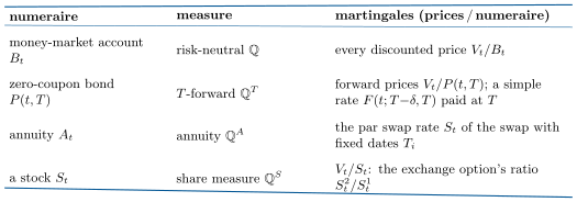
Geman, El Karoui and Rochet (1995) made this a working tool. The art is to choose the numeraire so that the ratio $V_T/\mathcal N_T$ is simple. Figure 5.2 lists the choices the series uses; Margrabe’s option to exchange one asset for another, priced with the second asset as numeraire, is Exercise 5.6.

**Figure 5.2.** Numeraires the series uses, their equivalent martingale measures, and what becomes a martingale under each: pricing a claim means choosing the numeraire that makes the claim’s ratio simplest.

5.4 The forward measure

Definition 5.7 (Forward measure)

The forward measure $\mathbb Q^T$ for maturity $T$ is the equivalent martingale measure for the numeraire $P(t, T)$ , the zero-coupon bond maturing at $T$ .

Proposition 5.8 (Discounting inside the expectation, and out)

For a payoff $X$ at $T$ : $\E^{\mathbb Q}_t[e^{-\int_t^Tr_s\,ds}X] = P(t, T)\,\E^{T}_t[X]$ . The forward price $V_t/P(t,T)$ of any traded asset is a $\mathbb Q^T$ -martingale, and in particular $\E^T[r_T] = f(0, T)$ , the instantaneous forward rate.

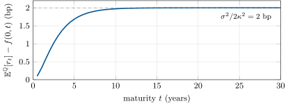
Proof. Apply the pricing formula with $\mathcal N = P(\cdot, T)$ , for which $P(T, T) = 1$ . For the last claim, $f(0,T) = -\partial_T\ln P(0,T) = \E^{\mathbb Q}[r_Te^{-\int_0^Tr}]/P(0,T) = \E^T[r_T]$ . ∎

The expectation of a stochastic discount factor times a payoff has become a deterministic discount factor times an expectation. For the Ornstein–Uhlenbeck short rate of chapter 4 ( $r_0 = 3\%$ , $\bar r = 4\%$ , $\kappa = 0.5$ , $\sigma = 1\%$ ), the bond has volatility $-\sigma B(T - t)$ , so by Theorem 5.6 the short rate’s drift under $\mathbb Q^T$ loses $\sigma^2B(T - t)$ : $r_T$ remains Gaussian, with a lower mean. $\E^{\mathbb Q}[r_5] = 3.918\%$ while $\E^5[r_5] = f(0, 5) = 3.901\%$ . The gap, a convexity effect, grows to $\sigma^2/2\kappa^2 = 2$ basis points at long maturities (Figure 5.3).

Expected short rate under the risk-neutral measure minus the instantaneous forward rate, which is the expected short rate under the forward measure of the same maturity, for the chapter’s Ornstein–Uhlenbeck short rate. The gap, 2B(t)2/2, is the price of the bond’s convexity. Data: closed forms, the chapter’s tutorial. — **Figure 5.3.** Expected short rate under the risk-neutral measure minus the instantaneous forward rate, which is the expected short rate under the forward measure of the same maturity, for the chapter’s Ornstein–Uhlenbeck short rate. The gap, $\sigma^2B(t)^2/2$ , is the price of the bond’s convexity. Data: closed forms, the chapter’s tutorial.

The caplet of the hook pays $\delta(F - K)^+$ at $T_1 + \delta$ on the rate $F$ fixed at $T_1 = 5$ for $\delta = \tfrac14$ year, with $K = 4.5\%$ . Its value at $T_1$ is $(1 + \delta K)(x - P(T_1, T_1 + \delta))^+$ with $x = 1/(1 + \delta K) = 0.98888$ : a put on a zero-coupon bond. Under $\mathbb Q^{T_1}$ , $P(T_1, T_1 + \delta) = e^{A - Br_{T_1}}$ is lognormal, and a Black-type formula follows (Jamshidian, 1989) with bond volatility $\sigma_P = \sigma\sqrt{(1 - e^{-2\kappa T_1})/2\kappa}\,B(\delta) = 0.234\%$ : 3.26 basis points of notional, USD 32 600 on USD 100 million. Figure 5.4 compares the two simulations.

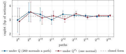
The caplet by Monte Carlo under the risk-neutral measure (weekly steps, money-market discounting) and under the fixing-date forward measure, with ± 2 standard errors, against the closed form 3.26 bp. At equal numbers of paths the errors are the same; the forward-measure path costs one normal instead of 260. Data: the chapter’s tutorial, seeded. — **Figure 5.4.** The caplet by Monte Carlo under the risk-neutral measure (weekly steps, money-market discounting) and under the fixing-date forward measure, with $\pm 2$ standard errors, against the closed form 3.26 bp. At equal numbers of paths the errors are the same; the forward-measure path costs one normal instead of 260. Data: the chapter’s tutorial, seeded.

The gain is not a smaller variance per path: the discount factor varies little next to the payoff, and the two standard errors per path are within half a percent of each other. It is the dimension of the problem, 260 normals down to one, and then no simulation at all.

5.5 The annuity measure

Definition 5.9 (Annuity measure)

For a swap with fixed payments at $T_1 < \dots < T_n$ and accrual fractions $\delta_i$ , the annuity measure $\mathbb Q^A$ is the equivalent martingale measure for the numeraire $A_t = \sum_i\delta_iP(t, T_i)$ , the annuity of One Quant Book 2, chapter 9.

The par swap rate is $S_t = (P(t, T_0) - P(t, T_n))/A_t$ , a traded value divided by the numeraire: a $\mathbb Q^A$ -martingale. A payer swaption exercised at $T_0$ pays $A_{T_0}(S_{T_0} - K)^+$ , so its value is $A_0\,\E^A[(S_{T_0} - K)^+]$ : with a normal law for $S_{T_0}$ this is the Bachelier formula of One Quant Book 2, chapter 13, with a lognormal one Black’s. The change of numeraire replaces a swaption, a claim on a whole curve, by a call on one martingale. One Quant Book 6 builds its rates models on this measure and on the forward measure.

5.6 Tutorial: two measures, one price

Goal. Price the caplet under two measures, check the reweighting between them, and see Girsanov at work on a histogram. End state: Figures 5.1, 5.3 and 5.4 and the price 3.26 bp.

The weights. The running project converts expectations between numeraires and builds Girsanov densities.

def change_of_numeraire_weights(m_T, m_0, n_T, n_0) -> np.ndarray:
    """dQ^M/dQ^N on each path: (M_T / M_0) / (N_T / N_0)."""
    return (np.asarray(m_T, float) / m_0) / (np.asarray(n_T, float) / n_0)


def reweighted_mean(x, w) -> tuple[float, float]:
    """E^M[X] = E^N[W X] estimated from samples under Q^N, with its standard error."""
    y = np.asarray(x, float) * np.asarray(w, float)
    return float(y.mean()), float(y.std(ddof=1) / math.sqrt(y.size))


def girsanov_weights(dw: np.ndarray, gamma, dt: float) -> np.ndarray:
    """Density exp(sum_k gamma_k dW_k - 1/2 sum_k gamma_k^2 dt) of the measure under which
    W - int gamma dt is a Brownian motion; `dw` has one row per path, `gamma` is a scalar, a
    per-step vector, or an array shaped like dw (it must be adapted: gamma_k known before dW_k)."""
    g = np.broadcast_to(np.asarray(gamma, float), dw.shape)
    return np.exp((g * dw).sum(axis=1) - 0.5 * (g**2).sum(axis=1) * dt)

Listing 5.1. Change-of-numeraire weights, a weighted mean, and a Girsanov density. code/firm/numeraire/firm_numeraire.py

The forward-measure sampler: the mean of $r_{T}$ loses $\sigma^2\int_0^Te^{-\kappa(T-s)}B(T - s)\,ds$ .

def forward_measure_moments(T=T1) -> tuple[float, float]:
    """Mean and variance of r_T under the T-forward measure: the drift loses sigma^2 B(T - t)."""
    shift = SIGMA**2 / KAPPA * ((1 - math.exp(-KAPPA * T)) / KAPPA - (1 - math.exp(-2 * KAPPA * T)) / (2 * KAPPA))
    var = SIGMA**2 * (1 - math.exp(-2 * KAPPA * T)) / (2 * KAPPA)
    return expected_short_rate(T) - shift, var


def mc_forward(n_paths: int, seed: int = 2, T=T1) -> dict:
    """Under Q^T: one Gaussian draw of r_T per path; price = P(0, T) E^T[payoff]."""
    rng = np.random.default_rng(seed)
    m, v = forward_measure_moments(T)
    r = m + math.sqrt(v) * rng.standard_normal(n_paths)
    y = float(zcb(R0, T)) * caplet_payoff_at_fixing(r)
    return {"price": float(y.mean()), "se": float(y.std(ddof=1) / math.sqrt(n_paths)), "normals": 1}

Listing 5.2. The short rate at the fixing date under the forward measure, and the caplet by one normal a path. code/methods/05-girsanov-and-changes-of-numeraire/python/qm_numeraire.py

Run problem(), reweighting_check() (100 000 risk-neutral paths reweighted by $d\mathbb Q^{T}/d\mathbb Q$ give $\E^{T}[r_5] = 3.906\% \pm 0.003\%$ against $3.901\%$ ) and fig_numeraire.py.

What to change next. Price the caplet under the payment-date measure $\mathbb Q^{T_1 + \delta}$ , under which the forward rate itself is a martingale; price a swaption under the annuity measure and compare with a risk-neutral simulation of the whole curve.

5.7 Build: moving between numeraires

Purpose. Every pricing engine of the miniature firm states its numeraire, and every simulated price is tested against it: a price divided by the numeraire must be a martingale.

Interface. change_of_numeraire_weights(m_T, m_0, n_T, n_0); reweighted_mean(x, w); girsanov_weights(dw, gamma, dt); deflated_martingale_test(prices, numeraire) returning the largest $|t|$ over dates.

Rules. Weights have mean one under the sampling measure (a test, not an assumption); the integrand of a Girsanov density is adapted; the martingale test uses paths simulated under the numeraire’s own measure.

Acceptance tests. code/firm/numeraire/tests/: Cameron–Martin weights shift a Gaussian’s mean and not its variance; reweighting risk-neutral short-rate paths reproduces the forward-measure mean; discounted bond prices pass the martingale test, undiscounted ones fail.

Stretch. The spot measure of a discretely rolled account (One Quant Book 6); likelihood-ratio sensitivities, which are Girsanov weights differentiated in a parameter (One Quant Book 5, chapter 23).

Sources and further reading

I. V. Girsanov, “On transforming a certain class of stochastic processes by absolutely continuous substitution of measures”, Theory of Probability and its Applications 5, 1960.
R. H. Cameron and W. T. Martin, “Transformations of Wiener integrals under translations”, Annals of Mathematics 45, 1944.
H. Geman, N. El Karoui and J.-C. Rochet, “Changes of numéraire, changes of probability measure and option pricing”, Journal of Applied Probability 32, 1995.
F. Jamshidian, “An exact bond option formula”, Journal of Finance 44, 1989.
W. Margrabe, “The value of an option to exchange one asset for another”, Journal of Finance 33, 1978.

5.8 Exercises

Exercise 5.1 ★

Under $d\mathbb Q/d\P = \exp(\gamma W_T - \gamma^2T/2)$ with $\gamma = 0.5$ and $T = 4$ , what is the law of $W_T$ ?

Solution

Solution of Exercise 5.1.

$W_T = W^{\mathbb Q}_T + \gamma T$ with $W^{\mathbb Q}$ a $\mathbb Q$ -Brownian motion: $W_T \sim \mathcal N(2, 4)$ under $\mathbb Q$ .

Exercise 5.2 ★

A stock has expected return 9% and volatility 25%, and the short rate is 4%. What is its drift under the risk-neutral measure, and what $\gamma$ does Girsanov use?

Solution

Solution of Exercise 5.2.

Drift 4%; $\gamma = -(\mu - r)/\sigma = -0.05/0.25 = -0.2$ , the negative of the Sharpe ratio.

Exercise 5.3 ★

A payoff at five years has $\E^{5}[X] = 2.4$ . With the chapter’s $P(0, 5)$ , what is it worth today?

Solution

Solution of Exercise 5.3.

$P(0,5)\,\E^5[X] = 0.8343 \times 2.4 = 2.002$ .

Exercise 5.4 ★★

Explain why $\E^{\mathbb Q}[r_T] > f(0, T)$ in the chapter’s model, and compute the gap at $T = 5$ from $\sigma^2B(T)^2/2$ .

Solution

Solution of Exercise 5.4.

Under $\mathbb Q^T$ the drift of $r$ loses $\sigma^2B(T - t) > 0$ : states with high rates, in which the bond is cheap, get less weight. $B(5) = 1.8358$ and $\sigma^2B^2/2 = 0.0001 \times 3.370/2 = 1.7$ bp, the gap between 3.918% and 3.901%.

Exercise 5.5 ★★

Show that the par swap rate is a martingale under the annuity measure, and write the value of a receiver swaption as an expectation under it.

Solution

Solution of Exercise 5.5.

$S_t = (P(t,T_0) - P(t,T_n))/A_t$ is a traded portfolio divided by the numeraire $A_t$ , hence a $\mathbb Q^A$ -martingale. A receiver swaption pays $A_{T_0}(K - S_{T_0})^+$ at $T_0$ , so its value is $A_0\,\E^A[(K - S_{T_0})^+]$ .

Exercise 5.6 ★★

Two stocks follow geometric Brownian motions with volatilities 20% and correlation 0.5, both at 100, no dividends. With the second as numeraire, price the option to receive the first in exchange for the second in one year.

Solution

Solution of Exercise 5.6.

Under $\mathbb Q^{S^2}$ the ratio $S^1/S^2$ is a martingale with volatility $\sqrt{0.2^2 + 0.2^2 - 2 \times 0.5 \times 0.04} = 0.2$ , and the value is $S^2_0\,\E^{S^2}[(S^1_T/S^2_T - 1)^+] = 100(\Phi(0.1) - \Phi(-0.1)) = 7.97$ : Margrabe’s formula, with no interest rate in it.

Exercise 5.7 ★★★

Derive the first-passage probability with drift of Proposition 2.9: remove the drift with Girsanov, apply the reflection principle’s joint law of the minimum and the end point, and integrate. Check it on the stop of chapter 2 with the drift $-\sigma^2/2$ .

Solution

Solution of Exercise 5.7.

Let $X = \mu t + \sigma W$ . Under $d\mathbb Q/d\P = e^{-(\mu/\sigma)W_T - \mu^2T/2\sigma^2}$ , $X/\sigma$ is a standard Brownian motion, and $d\P/d\mathbb Q = e^{(\mu/\sigma^2)X_T - \mu^2T/2\sigma^2}$ depends on the path only through $X_T$ . With $m = \min_{t\le T}X_t$ and $b < 0$ , the reflection principle gives under $\mathbb Q$ the joint law $\mathbb Q(m \le b, X_T \in dx) = \mathbb Q(X_T \in 2b - dx)$ for $x \ge b$ . Hence

\P(m \le b) = \P(X_T \le b) + \int_b^\infty e^{\mu x/\sigma^2 - \mu^2T/2\sigma^2}\,\varphi_{\sigma\sqrt T}(2b - x)\,dx,

where $\varphi_s$ is the $\mathcal N(0, s^2)$ density; completing the square, the integral is $e^{2\mu b/\sigma^2}\Phi((b + \mu T)/\sigma\sqrt T)$ , and $\P(X_T \le b) = \Phi((b - \mu T)/\sigma\sqrt T)$ . For the stop of chapter 2 ( $b = \ln 0.98$ , $\mu = -0.045$ , $\sigma = 0.30$ , $T = 21/252$ ): 82.4%.

Exercise 5.8 ★★★

Find the flaw. “To price the option we simulate the stock with our research team’s forecast drift of 12% a year and discount the payoffs at the risk-free rate: the forecast is our edge.”

Solution

Solution of Exercise 5.8.

A price is an expectation under a martingale measure for the chosen numeraire, not under the real-world measure: with the money-market account as numeraire the stock must drift at the short rate. Using the forecast drift prices a different, arbitrageable claim; the forecast belongs in the trading decision (buy if the market price is below the value one’s view implies), not in the pricing measure.

5.9 Problem: Two Measures, One Price

Problem 5.1

Weekend problem — a five-year caplet, two ways

The short rate is $dr = \kappa(\bar r - r)\,dt + \sigma\,dW^{\mathbb Q}$ with $r_0 = 3\%$ , $\bar r = 4\%$ , $\kappa = 0.5$ and $\sigma = 1\%$ . A caplet fixes at $T_1 = 5$ on the rate for $[5, 5.25]$ , pays at 5.25, strike 4.5%, notional USD 100 million.

Part I — The curve.

What are $P(0, 5)$ and $P(0, 5.25)$ ?
What is the forward rate for $[5, 5.25]$ ?
What are $\E^{\mathbb Q}[r_5]$ and $f(0, 5)$ , and why do they differ?
Write the caplet as a put on a zero-coupon bond: strike and number of bonds.
What is the bond volatility $\sigma_P$ in Jamshidian’s formula?

Part II — Three prices.

What does the closed form give, in basis points and in dollars?
How many normals does a risk-neutral path with weekly steps use, and a forward-measure path?
What do 20 000 risk-neutral paths give, with standard error?
And 20 000 forward-measure paths?
Are the two within their standard errors of the closed form?

Part III — What the measure change bought.

What is the density $d\mathbb Q^{T_1}/d\mathbb Q$ on a path?
What does reweighting 100 000 risk-neutral paths give for $\E^{T_1}[r_5]$ ?
What is the ratio of the two standard errors at equal paths, and why is it close to one?
What, then, is the gain at equal accuracy?
With four times finer steps under $\mathbb Q$ , does the risk-neutral price change?

Part IV — Judgement.

A cap is a strip of caplets with different payment dates. Which measure do you use?
Which measure prices a swaption, and what becomes a martingale?
What should a pricing library’s acceptance test check about its numeraire?
State the named result: the caplet’s price and what the forward measure bought.
In one sentence: what does a change of numeraire change, and what does it not?

Solution

Solution of Problem 5.1.

1. $P(0,5) = 0.8343$ , $P(0,5.25) = 0.8262$ . 2. $(0.8343/0.8262 - 1)/0.25 = 3.92\%$ . 3. 3.918% and 3.901%: under the forward measure the drift of $r$ is lower by $\sigma^2B(5 - t)$ . 4. A put struck at $x = 1/(1 + \delta K) = 0.98888$ on $1 + \delta K = 1.01125$ zero-coupon bonds maturing at 5.25, expiring at 5. 5. $\sigma_P = 0.01\sqrt{(1 - e^{-5})/1}\times B(0.25) = 0.234\%$ . 6. 3.26 bp of notional: USD 32 600. 7. 260 (weekly steps over five years) against one. 8. $3.34 \pm 0.05$ bp. 9. $3.32 \pm 0.05$ bp. 10. Yes: 1.6 and 1.2 standard errors from 3.26. 11. $(P(5,5)/P(0,5))/(B_5/B_0) = 1/(P(0,5)B_5)$ , with $B_5 = e^{\int_0^5r}$ along the path. 12. $3.906\% \pm 0.003\%$ , against $f(0,5) = 3.901\%$ ; the weights average 1.000. 13. 0.996: the discount factor’s randomness is small next to the payoff’s, so removing it barely reduces the variance per path. 14. The cost per path: one normal instead of 260, so about 260 times less work for the same error, and then the closed form with none. 15. No: $3.32 \pm 0.05$ bp with 208 steps a year, within noise of 3.34. 16. Each caplet under the forward measure of its own date, then sum; a joint simulation of all dates needs one measure for all, the spot or terminal measure of One Quant Book 6. 17. The annuity measure; the par swap rate is its martingale. 18. That every simulated price divided by the numeraire has a constant mean over dates (the deflated martingale test), and that change-of-numeraire weights average one. 19. Named result: two measures, one price: the caplet is worth 3.26 bp of notional (USD 32 600 on USD 100 million); risk-neutral and forward-measure simulations agree with it and have the same standard error per path, but the forward measure needs one normal a path instead of 260, and yields the closed form. 20. It changes the drift and the unit in which values are counted, never the prices and never the volatility.

5.10 Interview questions

Interview question 5.1 ★ researcher, bank

What does Girsanov’s theorem change about a Brownian motion, and what can it not change?

Solution

Solution of Interview question 5.1.

It adds a drift: $W - \int\gamma\,dt$ is a Brownian motion under the new measure. It cannot change the quadratic variation, which is visible on a single path, so volatilities are the same under all equivalent measures.

What the interviewer is looking for: drift yes, volatility no, and why.

Interview question 5.2 ★ bank, trader

Why does a stock drift at the risk-free rate under the risk-neutral measure, when nobody expects it to?

Solution

Solution of Interview question 5.2.

The risk-neutral measure is a pricing device, not a forecast: it is the measure under which prices counted in units of the money-market account are fair games. A stock held against a short money-market position must then earn nothing on average in those units, so its drift is $r$ ; the real expected return lives under $\P$ .

What the interviewer is looking for: measure as a unit of account, not a belief.

Interview question 5.3 ★★ bank

What is the forward measure, and why is the forward rate a martingale under it?

Solution

Solution of Interview question 5.3.

The equivalent martingale measure for the zero-coupon bond maturing at $T$ . The simple forward rate for $[S, T]$ is $(P(t,S)/P(t,T) - 1)/\delta$ : a traded price divided by the numeraire, minus a constant, hence a martingale.

What the interviewer is looking for: numeraire $P(t,T)$ and the ratio argument.

Interview question 5.4 ★★ bank, researcher

Price the option to exchange asset 2 for asset 1 at $T$ . Which numeraire, and why?

Solution

Solution of Interview question 5.4.

With asset 2 as numeraire the payoff $(S^1_T - S^2_T)^+ = S^2_T(S^1_T/S^2_T - 1)^+$ becomes a call on the martingale $S^1/S^2$ struck at one, with volatility $\sqrt{\sigma_1^2 + \sigma_2^2 - 2\rho\sigma_1\sigma_2}$ : Margrabe’s formula, independent of rates.

What the interviewer is looking for: choosing the numeraire that removes one asset.

Interview question 5.5 ★★ developer, bank

How would you test that a Monte Carlo pricing engine uses a consistent measure?

Solution

Solution of Interview question 5.5.

Simulate traded instruments whose prices are known (zero-coupon bonds, forwards) and check that their prices divided by the engine’s numeraire have constant means over all dates within a few standard errors; check put–call parity on the simulated payoffs; and price the same claim under two numeraires with the reweighting.

What the interviewer is looking for: martingale tests on instruments with known prices.

Interview question 5.6 ★★★ researcher

Estimate $\P(W_1 > 5)$ by simulation with fewer than 10 000 draws.

Solution

Solution of Interview question 5.6.

Plain sampling sees an exceedance once in 3.5 million draws. Sample $Y \sim \mathcal N(5, 1)$ instead and average $e^{-5Y + 12.5}\mathbf 1_{\{Y > 5\}}$ : 10 000 draws give $2.79 \times 10^{-7}$ with a standard error of $0.07 \times 10^{-7}$ , against the exact $2.87 \times 10^{-7}$ .

What the interviewer is looking for: importance sampling by a mean shift, with the likelihood-ratio weight.

Terms defined in this chapter

See all 2333 terms in the glossary