9Stochastic Control

After a 20% fall in equities a pension fund’s equity weight has drifted from 60% to 52%. Its rulebook says: rebalance to 60% at the quarter-end, which means buying equities after a fall. Half the investment committee wants to wait for the market to settle. The question is one of stochastic control: choose, at each moment and with what is known then, how much to hold, so as to maximise the expected utility of what the fund ends with. For an investor with constant relative risk aversion in a market of lognormal prices, Merton solved it in 1969: hold a constant fraction, whatever has happened, and rebalance to it. With this fund’s assumptions the fraction is 51%, holding 60% instead costs 3.6 basis points of certainty-equivalent return a year, and the committee’s debate is about a much smaller number than the uncertainty in its own expected return. This chapter develops dynamic programming in discrete time, the Hamilton–Jacobi–Bellman equation in continuous time, the verification theorem that turns a candidate into a proof, Merton’s problem, and a sketch of the viscosity solutions that handle value functions with kinks.

9.1 Dynamic programming

Definition 9.1 (Stochastic control problem, admissible control, value function)

A stochastic control problem chooses a process $u_t$ that influences the dynamics of a state $X$, here $dX_t = \mu(t, X_t, u_t)\,dt + \sigma(t, X_t, u_t)\,dW_t$ or its discrete-time analogue, to maximise $J(t, x; u) = \E_{t,x}[\int_t^Tf(s, X_s, u_s)\,ds + g(X_T)]$. An admissible control is an adapted process with values in a set $\mathcal U$ for which the state equation has a solution and $J$ is well defined. The value function is $V(t, x) = \sup_uJ(t, x; u)$ over admissible controls.

Theorem 9.2 (Dynamic programming principle)

For every $t < s \le T$, $V(t, x) = \sup_u\E_{t,x}\bigl[\int_t^sf(r, X_r, u_r)\,dr + V(s, X_s)\bigr]$.

Definition 9.3 (Dynamic programming, feedback control)

Dynamic programming computes the value function backward in time with the one-step principle, $V_t(x) = \max_u\{f(t, x, u) + \E[V_{t+1}(X_{t+1}) \mid X_t = x, u]\}$, from $V_T = g$. A feedback control is a control of the form $u_t = u^*(t, X_t)$, a function of the current state; dynamic programming produces one.

The principle reduces a choice over whole strategies to a sequence of one-step choices, at the cost of computing $V$ on the whole state space: the curse of dimensionality. The running project’s solver (the tutorial’s first listing) does it on a grid, with the expectation computed by quadrature over the next state and linear interpolation between grid points.

9.2 The Hamilton–Jacobi–Bellman equation

Definition 9.4 (Hamilton–Jacobi–Bellman equation)

For the controlled diffusion of Definition 9.1, the Hamilton–Jacobi–Bellman equation is

$$\partial_tV(t, x) + \sup_{u\in\mathcal U}\Bigl\{\mu(t, x, u)\partial_xV + \tfrac12\sigma^2(t, x, u)\partial_{xx}V + f(t, x, u)\Bigr\} = 0, \qquad V(T, x) = g(x).$$

It is the dynamic programming principle over an interval $[t, t + h]$ with $h \to 0$: expand $V(t + h, X_{t+h})$ by Itô’s formula, take expectations, divide by $h$. For each fixed control it is the backward equation of chapter 4 with the generator $\mathcal L^u$ of the controlled state; the supremum makes it nonlinear. The heuristic assumes $V$ is smooth, which is what the verification theorem replaces by an assumption about a candidate.

9.3 Verification

Theorem 9.5 (Verification)

Let $w \in C^{1,2}$ with polynomial growth solve the HJB equation, and suppose the supremum is attained at $u^*(t, x)$ such that the state equation with the feedback $u^*$ has a solution. Then $w = V$ and $u^*$ is optimal, provided the stochastic integrals below are true martingales.

9.4 Merton’s problem

Definition 9.6 (Utility function, relative risk aversion, CRRA utility)

A utility function $U$ is increasing and concave; the investor maximises $\E[U(W_T)]$. Its relative risk aversion is $-wU^{\prime\prime}(w)/U'(w)$. CRRA utility has constant relative risk aversion $\gamma > 0$: $U(w) = w^{1-\gamma}/(1 - \gamma)$, and $\ln w$ for $\gamma = 1$.

Definition 9.7 (Certainty equivalent)

The certainty equivalent of a random wealth $W$ is the sure amount $c$ with $U(c) = \E[U(W)]$; over a horizon $T$, the certainty-equivalent return is $\ln(c/W_0)/T$.

A fund holds a fraction $\pi_t$ of its wealth in a stock with $dS/S = \mu\,dt + \sigma\,dW$ and the rest in the money-market account at rate $r$, so $dW_t = W_t(r + \pi_t(\mu - r))\,dt + W_t\pi_t\sigma\,dW_t$.

Theorem 9.8 (Merton)

For CRRA utility of terminal wealth, the optimal fraction is constant,

$$\pi^* = \frac{\mu - r}{\gamma\sigma^2},$$

and the value function is $V(t, w) = \frac{w^{1-\gamma}}{1-\gamma}e^{(1-\gamma)\rho(T-t)}$, where $\rho = r + \frac{(\mu - r)^2}{2\gamma\sigma^2}$ is the certainty-equivalent return of the optimal strategy.

Definition 9.9 (Merton fraction)

The Merton fraction is $\pi^* = (\mu - r)/(\gamma\sigma^2)$.

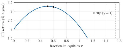
The optimal fraction does not depend on wealth or on time: after a fall the fund should buy back to it. Holding a constant $\pi$ earns the certainty-equivalent return $r + \pi(\mu - r) - \tfrac12\gamma\pi^2\sigma^2$ (Figure 9.1), so a mistaken fraction costs $\tfrac12\gamma\sigma^2(\pi - \pi^*)^2$ a year. With $\mu = 7\%$, $r = 2\%$, $\sigma = 18\%$ and $\gamma = 3$: $\pi^* = 51.4\%$, a certainty-equivalent return of 3.29%, and 60% costs 3.6 basis points a year. With $\gamma = 1$, log utility, $\pi^* = (\mu - r)/\sigma^2$ is the Kelly fraction of One Quant Book 2, chapter 29, here 154%: the growth-optimal investor borrows.

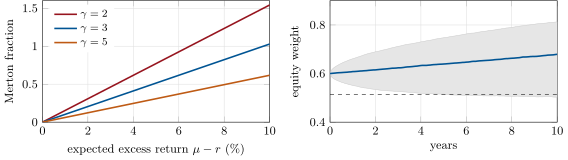
The flatness has a flip side. The fraction is proportional to the expected excess return, which is known far less well: estimated from ten years of returns with 18% volatility, $\mu$ has a standard error of $18\%/\sqrt{10} = 5.7\%$, and every point of $\mu$ moves $\pi^*$ by ten points (Figure 9.2). Merton’s rule is exact and its input is uncertain; chapter 14 shrinks the input.

9.5 A sketch of viscosity solutions

Value functions are often not smooth: a control that switches from one extreme to another at a boundary puts a kink in $V$, and the HJB equation cannot hold there in the classical sense. The right notion replaces derivatives by smooth test functions touching $V$.

Definition 9.10 (Viscosity solution)

A continuous $V$ is a viscosity solution of $F(x, V, DV, D^2V) = 0$ ($F$ nonincreasing in its last argument) if at every point where a smooth $\phi$ touches $V$ from above ($V - \phi$ has a local maximum), $F(x, V, D\phi, D^2\phi) \le 0$, and at every point where it touches from below, $F \ge 0$.

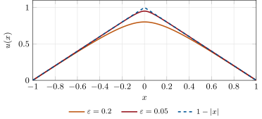
For the problem of leaving $(-1, 1)$ as fast as possible at unit speed, $V(x) = 1 - |x|$ and $|V'| = 1$ everywhere but at zero, where no derivative exists; it is the viscosity solution, and it is the limit as $\varepsilon \to 0$ of the smooth solutions of $-\varepsilon u^{\prime\prime} + |u'| = 1$ (Figure 9.3), which is where the name comes from. Crandall and Lions (1983) proved existence and uniqueness for first-order equations; the theory guarantees that dynamic programming on a grid converges to the right value function even when it has kinks, as in the stopping problems of chapter 10.

9.6 Tutorial: Merton by backward induction

9.7 Build: the dynamic-programming solver

9.8 Exercises

Exercise 9.1 ★

An asset has an expected excess return of 4% and a volatility of 20%. What fraction does an investor with $\gamma = 4$ hold?

Solution

Solution of Exercise 9.1.

$0.04/(4 \times 0.04) = 25\%$.

Exercise 9.2 ★

With the fund’s assumptions, what is the certainty-equivalent return of holding 100% in equities?

Solution

Solution of Exercise 9.2.

$0.02 + 0.05 - \tfrac12 \times 3 \times 0.0324 = 2.14\%$ a year, against 3.29% at the optimum.

Exercise 9.3 ★

Compute the relative risk aversion of $U(w) = \ln w$ and of $U(w) = w^{1-\gamma}/(1 - \gamma)$.

Solution

Solution of Exercise 9.3.

For $\ln w$: $-w(-1/w^2)/(1/w) = 1$. For $w^{1-\gamma}/(1 - \gamma)$: $-w(-\gamma w^{-\gamma-1})/w^{-\gamma} = \gamma$.

Exercise 9.4 ★★

Show that holding a constant $\pi$ instead of $\pi^*$ costs $\tfrac12\gamma\sigma^2(\pi - \pi^*)^2$ of certainty-equivalent return a year, and evaluate it for 60% against 51.4%.

Solution

Solution of Exercise 9.4.

The certainty-equivalent return $c(\pi) = r + \pi(\mu - r) - \tfrac12\gamma\pi^2\sigma^2$ is a parabola with maximum at $\pi^*$ and second derivative $-\gamma\sigma^2$, so $c(\pi^*) - c(\pi) = \tfrac12\gamma\sigma^2(\pi - \pi^*)^2 = \tfrac12 \times 3 \times 0.0324 \times 0.0856^2 = 3.6$ bp.

Exercise 9.5 ★★

What fraction does a log-utility investor hold with the fund’s assumptions? Why would a fund not do so?

Solution

Solution of Exercise 9.5.

$0.05/0.0324 = 154\%$, borrowing 54% of wealth. The fund’s risk aversion is higher than log utility, the expected return is uncertain (overbetting costs more than underbetting, One Quant Book 2, chapter 29), and leverage brings margin and drawdown constraints the model ignores.

Exercise 9.6 ★★

Verify that $V = \frac{w^{1-\gamma}}{1-\gamma}e^{(1-\gamma)\rho(T-t)}$ solves the HJB equation, with $\rho = r + (\mu - r)^2/(2\gamma\sigma^2)$, and compute $\rho$ for the fund.

Solution

Solution of Exercise 9.6.

From the proof of Theorem 9.8: $\partial_tV = -(1 - \gamma)\rho V$ and the supremum is $(1 - \gamma)\rho V$, so the equation holds. For the fund, $\rho = 0.02 + 0.05^2/(2 \times 3 \times 0.0324) = 3.29\%$.

Exercise 9.7 ★★★

Coding. With backward_induction, solve the fund’s problem with $\gamma = 5$ and annual rebalancing. Is the fraction still independent of wealth, and how does it compare with $(\mu - r)/(\gamma\sigma^2)$?

Solution

Solution of Exercise 9.7.

Yes: 0.315 at every wealth level, against $(\mu - r)/(\gamma\sigma^2) = 0.309$ and a one-period optimum of 0.309; the small gap comes from interpolating the value function on the grid.

Exercise 9.8 ★★★

Find the flaw. “We estimated the equity premium at 5% from ten years of data, so our optimal equity weight is 51%, and we will hold exactly that.”

Solution

Solution of Exercise 9.8.

Ten years of returns with 18% volatility estimate the premium with a standard error of $18\%/\sqrt{10} = 5.7\%$, which moves the Merton fraction by $\pm 59$ points: the data cannot distinguish 0% from 100%. Shrink the estimate toward a prior (chapter 14) and size for the uncertainty, not for the point estimate.

9.9 Problem: The Rebalancing Committee

Problem 9.1

Weekend problem — how much the committee’s decision is worth

A fund with CRRA utility, $\gamma = 3$, expects equities to return $\mu = 7\%$ with volatility $\sigma = 18\%$; cash earns $r = 2\%$. Its rulebook holds 60% in equities, rebalanced. After a fall its weight is 52%.

Part I — Merton.

1. What is the Merton fraction?
2. What is the certainty-equivalent return of the optimal strategy?
3. What does holding 60% cost a year?
4. And holding 52%?
5. What trade does Merton recommend after the fall, and what does the rulebook recommend?

Part II — Sensitivity.

6. What are the fractions for $\gamma = 2$ and $\gamma = 5$?
7. And for $\mu = 6\%$ and $8\%$?
8. What does $\gamma = 1$ give, and what does it mean?
9. What does the grid dynamic programme with annual rebalancing give, and the one-period optimum?
10. Why does the fraction not depend on wealth?

Part III — Rebalancing.

11. Over ten simulated years, what certainty-equivalent returns do constant 60%, Merton, and buy-and-hold from 60% achieve?
12. Where does the buy-and-hold weight end after ten years (10th percentile, median, 90th)?
13. What does never rebalancing cost, against rebalancing to 60%?
14. With what standard error is $\mu$ known from ten years of returns, and what band does that put on $\pi^*$?
15. Which matters more for the fund: the committee’s choice between 52% and 60%, or the uncertainty in $\mu$?

Part IV — Judgement.

16. What would transaction costs change?
17. What would liabilities (a pension promise) change?
18. What should the chief investment officer tell the committee?
19. State the named result: the Merton fraction and the cost of the rulebook’s 60%.
20. In one sentence: what does Merton’s solution say about rebalancing after a fall?

Solution

Solution of Problem 9.1.

1. $0.05/(3 \times 0.0324) = 51.4\%$. 2. $\rho = 3.29\%$. 3. 3.6 bp a year. 4. 0.02 bp: 52% is almost exactly optimal. 5. Merton: sell 0.6 point, practically nothing; the rulebook: buy 8 points back to 60%. 6. 77% and 31%. 7. 41% and 62%. 8. 154%: the Kelly, growth-optimal fraction, with borrowing. 9. 0.52 at every wealth level and date; the one-period optimum is 0.517 (continuous: 0.514). 10. CRRA utility is homothetic: scaling wealth scales utility, so the best fraction is the same at every wealth. 11. 3.28%, 3.31% and 3.24% (theory for Merton: 3.29%). 12. 50%, 68% and 81%. 13. 3.3 bp a year. 14. 5.7%; $\pi^*$ moves by $0.057/(3 \times 0.0324) = 59$ points either way, from about $-7\%$ to $110\%$. 15. The uncertainty in $\mu$, by far: the committee is debating a few basis points of certainty equivalent. 16. A band around the target inside which the fund does not trade (chapter 10). 17. The fund would hold a liability-hedging portfolio plus a Merton-like position whose size depends on its funding surplus; the fraction would depend on wealth. 18. Rebalance mechanically to a target; spend the debate on the inputs (expected return, risk aversion) and on costs, not on timing. 19. Named result: the rebalancing committee: the Merton fraction is 51.4%; holding the rulebook’s 60% costs 3.6 bp a year of certainty-equivalent return, never rebalancing about 3.3 bp, and one standard error in the expected return moves the fraction by 59 points. 20. Rebalance back to the constant fraction, since nothing about the optimum changed with the price.

9.10 Interview questions

Interview question 9.1 ★ researcher, trader

State Merton’s optimal fraction and explain each of its three inputs.

Solution

Solution of Interview question 9.1.

$\pi^* = (\mu - r)/(\gamma\sigma^2)$: the expected excess return (more reward, more stock), risk aversion (more aversion, less), and variance (more risk, less): a mean-variance trade-off per unit of wealth.

What the interviewer is looking for: the formula and its comparative statics.

Interview question 9.2 ★★ researcher

Derive the HJB equation from the dynamic programming principle.

Solution

Solution of Interview question 9.2.

$V(t, x) = \sup_u\E[\int_t^{t+h}f\,ds + V(t + h, X_{t+h})]$; expand $V(t + h, X_{t+h})$ by Itô, take expectations, subtract $V(t, x)$, divide by $h$ and let $h \to 0$: $\partial_tV + \sup_u\{\mathcal L^uV + f\} = 0$.

What the interviewer is looking for: Itô inside the dynamic programming principle.

Interview question 9.3 ★★ researcher

Why does a CRRA investor in Merton’s model buy equities after they fall?

Solution

Solution of Interview question 9.3.

The optimal fraction is constant; a fall lowers the equity share below it, so restoring it means buying. Nothing in the model’s opportunity set changed with the price: returns are independent and identically distributed.

What the interviewer is looking for: constant fraction plus i.i.d. returns.

Interview question 9.4 ★★ trader, researcher

How does the Kelly criterion relate to Merton’s problem?

Solution

Solution of Interview question 9.4.

Kelly maximises expected log wealth: Merton with $\gamma = 1$, giving $(\mu - r)/\sigma^2$. More risk-averse investors hold a fraction $1/\gamma$ of it: fractional Kelly is Merton with $\gamma > 1$.

What the interviewer is looking for: log utility and fractional Kelly.

Interview question 9.5 ★★ developer

Your dynamic programme on a grid returns a policy that jumps between neighbouring grid points. What do you check?

Solution

Solution of Interview question 9.5.

Whether the objective is flat there (then the choice barely matters), the control grid is too coarse, the quadrature too crude, or the interpolation of the value function too rough; refine each and see whether the policy converges.

What the interviewer is looking for: flatness versus numerical error, and a convergence check.

Interview question 9.6 ★★★ researcher

When is the value function of a control problem not smooth, and how does one make sense of the HJB equation then?

Solution

Solution of Interview question 9.6.

When the optimal control switches between extremes, or at a stopping boundary, or with degenerate diffusion: the value function has kinks. It is then the unique viscosity solution: at every point, smooth functions touching it from above or below satisfy the equation’s inequalities, which is also the notion under which grid schemes converge.

What the interviewer is looking for: test functions touching from above and below.