11Estimation

A researcher presents a strategy: over five years its daily P&L averaged 4.0 basis points with a standard error of 1.2, a $t$-statistic of 3.4, comfortably significant. A colleague notices that each day’s position is held for five days, so consecutive days share four fifths of their positions, and recomputes the standard error allowing for the autocorrelation that creates: 2.3. The $t$-statistic falls to 1.7, and the strategy is no longer distinguishable from luck. Nothing was wrong with the average; the formula for its uncertainty assumed independent days. This chapter is about estimators and their uncertainty: maximum likelihood and its asymptotics, what happens when the model is wrong, M-estimators and moments, the delta method that gives the Sharpe ratio its standard error, and the heteroskedasticity- and autocorrelation-consistent variances that repaired the researcher’s $t$-statistic.

11.1 Maximum likelihood

Definition 11.1 (Estimator, unbiased, consistent, standard error)

An estimator $\hat\theta_n$ of a parameter $\theta_0$ is a function of the data $X_1, \dots, X_n$. It is an unbiased estimator if $\E[\hat\theta_n] = \theta_0$, and a consistent estimator if $\hat\theta_n \xrightarrow{\P} \theta_0$ as $n \to \infty$. Its standard error $\mathrm{se}(\hat\theta_n)$ is (an estimate of) its standard deviation.

The sample variance with divisor $n$ is biased and consistent; with divisor $n - 1$ it is unbiased. Consistency is what matters with the sample sizes of finance, and so does the standard error: an estimate without one is an anecdote.

Definition 11.2 (Likelihood function, maximum likelihood estimator, score, Fisher information)

For independent observations with density $f(x; \theta)$, the likelihood function is $\theta \mapsto \prod_if(X_i; \theta)$ and the log-likelihood $\ell_n(\theta) = \sum_i\ln f(X_i; \theta)$. The maximum likelihood estimator (MLE) maximises it. The score function is $\nabla_\theta\ln f(X; \theta)$, and the Fisher information is $\mathcal I(\theta) = \E[\nabla\ln f\,\nabla\ln f^\top] = -\E[\nabla^2\ln f]$ per observation.

Theorem 11.3 (Asymptotics of maximum likelihood)

Under regularity conditions (identifiability, smoothness, a true value in the interior), the MLE is consistent and

$$\sqrt n(\hat\theta_n - \theta_0) \xrightarrow{d} \mathcal N\bigl(0, \mathcal I(\theta_0)^{-1}\bigr).$$

No unbiased estimator has a smaller variance than $\mathcal I(\theta_0)^{-1}/n$ (the Cramér–Rao bound), so the MLE is asymptotically efficient.

Example 11.4 (The rate of arrivals)

For $n$ exponential waiting times with rate $\lambda$, $\ell_n(\lambda) = n\ln\lambda - \lambda\sum t_i$, so $\hat\lambda = n/\sum t_i$, $\mathcal I(\lambda) = 1/\lambda^2$, and $\mathrm{se}(\hat\lambda) = \hat\lambda/\sqrt n$. A hundred gaps summing to 50 seconds give $2 \pm 0.2$ arrivals per second. The Hawkes fits of chapter 7 are the same computation with a harder likelihood.

11.2 Misspecification and the sandwich

Models are approximations; the question is what maximum likelihood estimates when the density is wrong.

Definition 11.5 (Kullback–Leibler divergence, quasi-maximum likelihood)

The Kullback–Leibler divergence of a density $f$ from the true density $p$ is $D_{\mathrm{KL}}(p\,\|\,f) = \E_p[\ln(p(X)/f(X))] \ge 0$, zero only if $f = p$. Quasi-maximum likelihood maximises a likelihood that is not believed to be the true one.

Proposition 11.6 (What a wrong likelihood estimates)

Under regularity conditions the quasi-MLE converges to the pseudo-true value $\theta^*$ that minimises $D_{\mathrm{KL}}(p\,\|\,f_\theta)$, and $\sqrt n(\hat\theta_n - \theta^*) \xrightarrow{d} \mathcal N(0, A^{-1}BA^{-1})$ with $A = -\E[\nabla^2\ln f_{\theta^*}]$ and $B = \Var(\nabla\ln f_{\theta^*})$.

Definition 11.7 (Sandwich variance)

The sandwich variance of an estimator defined by an estimating equation is $A^{-1}BA^{-1}$: the bread $A$, the expected derivative of the estimating equation, around the meat $B$, the variance of the equation itself. Estimated by the sample Hessian and the outer product of the per-observation scores, it is the robust (Huber–White) variance.

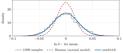
Fit a normal model to 2 000 draws of a Student $t$ with 6 degrees of freedom. The estimate of the log standard deviation is still consistent for the log standard deviation, but the Hessian standard error, 0.0158, assumes normal tails; the sandwich gives 0.0230, and over 4 000 simulated samples the actual spread is 0.0237 (Figure 11.1). With fatter tails still (4 degrees of freedom, infinite fourth moment) the variance of the sample variance does not exist, and no standard error is right.

11.3 M-estimators and the method of moments

Definition 11.8 (M-estimator, method of moments, generalised method of moments)

An M-estimator maximises (or zeroes the derivative of) a sample average $n^{-1}\sum_im(X_i; \theta)$; maximum likelihood takes $m = \ln f$, least squares $m = -(y - x^\top\theta)^2$. The method of moments solves $n^{-1}\sum_ig(X_i) = \E_\theta[g(X)]$ for as many moments as parameters. The generalised method of moments (GMM) minimises $\bar g_n(\theta)^\top W\bar g_n(\theta)$ for $\bar g_n(\theta) = n^{-1}\sum_ig(X_i; \theta)$ with more moment conditions than parameters and a weight matrix $W$.

All three have the sandwich asymptotics of Proposition 11.6, with $A$ the derivative of the estimating equations and $B$ their long-run variance; GMM is efficient when $W$ is the inverse of that variance (Hansen, 1982), and the minimised objective then tests the overidentifying conditions. For an Ornstein–Uhlenbeck process sampled daily, the method of moments on the first autocorrelation, $\hat\kappa = -\ln\hat\rho(1)/\Delta t$, coincides with the conditional maximum likelihood of the autoregression (chapter 17), and both inherit its small-sample bias.

11.4 The delta method and the Sharpe ratio

Method 11.9 (Delta method)

If $\sqrt n(\hat\theta_n - \theta_0) \xrightarrow{d} \mathcal N(0, V)$ and $g$ is differentiable at $\theta_0$, then $\sqrt n(g(\hat\theta_n) - g(\theta_0)) \xrightarrow{d} \mathcal N(0, \nabla g^\top V\nabla g)$. The delta method linearises a smooth function of an estimate and propagates its variance.

Definition 11.10 (Sharpe ratio)

The Sharpe ratio of a strategy is its expected excess return per unit of standard deviation, $\mathrm{SR} = \mu/\sigma$, per period; annualised by $\sqrt{\text{periods a year}}$ when returns are independent across periods. Its estimate is $\widehat{\mathrm{SR}} = \bar x/s$.

Proposition 11.11 (Standard error of the Sharpe ratio)

For independent normal returns, $\sqrt n(\widehat{\mathrm{SR}} - \mathrm{SR}) \xrightarrow{d} \mathcal N(0, 1 + \tfrac12\mathrm{SR}^2)$ per period.

Annualised, the standard error is about $\sqrt{(1 + \mathrm{SR}_1^2/2)/\text{years}}$, since the per-day Sharpe ratio $\mathrm{SR}_1$ is small: five years estimate an annual Sharpe ratio to $\pm 0.45$, whatever its size. The researcher’s strategy has $\widehat{\mathrm{SR}} = 1.51$ with that standard error under independence (Lo, 2002, derives the general case). With non-normal returns $B$ changes; with autocorrelated returns, the annualisation by $\sqrt{252}$ and the variance both change, which is the next section’s subject: the HAC version of the same delta method gives 0.87.

11.5 Serial correlation: HAC variances

The mean of a stationary series with autocovariances $\gamma(k)$ has

The researcher’s P&L is the average of five overlapping five-day positions, so its autocorrelations are $1 - k/5$ for $k \le 4$ (Figure 11.2), and the long-run variance is $1 + 2(0.8 + 0.6 + 0.4 + 0.2) = 5$ times the variance: the naive standard error is $\sqrt5 = 2.24$ times too small.

Definition 11.12 (HAC estimator)

A heteroskedasticity- and autocorrelation-consistent (HAC estimator) estimates a long-run variance by weighting sample autocovariances; the Newey–West estimator $\hat\gamma(0) + 2\sum_{k=1}^L(1 - \frac k{L+1})\hat\gamma(k)$ uses Bartlett weights, which keep it nonnegative, with a bandwidth $L$ growing slowly with $n$ (a common rule is $L = \lfloor4(n/100)^{2/9}\rfloor$).

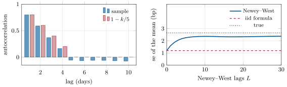
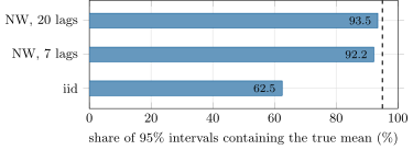
With seven lags, Newey–West gives 2.32 basis points and a $t$-statistic of 1.73: the colleague’s number. It still understates the true 2.65, because the estimated autocovariances are biased toward zero in a sample of 1 260 days. Over 2 000 simulated histories of the strategy, nominal 95% intervals built on the iid standard error contain the true mean 62.5% of the time; with Newey–West, 92.2% with seven lags and 93.5% with twenty (Figure 11.3). A HAC standard error is necessary, not sufficient; the model-based alternative, when the overlap is known, uses the factor 5 directly.

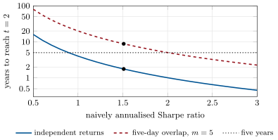
The same arithmetic tells a researcher how long to wait. An annual Sharpe ratio $\mathrm{SR}$ estimated from independent daily returns reaches a $t$-statistic of 2 after about $4/\mathrm{SR}^2$ years: one year at a Sharpe ratio of 2, four at 1, sixteen at 0.5. If the long-run variance is $m$ times the variance, as with the overlapping positions ($m = 5$), the naive annualisation overstates the Sharpe ratio by $\sqrt m$ and the wait is $m$ times longer (Figure 11.4): the researcher’s naive 1.51 needs 1.8 years, the honest reading 8.8. Five years of history cannot separate an honest Sharpe ratio of 0.68 from zero.

11.6 Tutorial: the $t$-statistic that halved

11.7 Build: the estimation toolkit

11.8 Exercises

Exercise 11.1 ★

A hundred waiting times between trades sum to 50 seconds. Estimate the arrival rate and its standard error.

Solution

Solution of Exercise 11.1.

$\hat\lambda = 100/50 = 2$ per second; $\mathrm{se} = \hat\lambda/\sqrt{100} = 0.2$.

Exercise 11.2 ★

A strategy’s annualised Sharpe ratio is estimated at 1.0 from four years of independent daily returns. What is its standard error?

Solution

Solution of Exercise 11.2.

Per day $\mathrm{SR}_1 = 1/\sqrt{252} = 0.063$ and $\mathrm{se} = \sqrt{(1 + 0.002)/1\,008} = 0.0315$; annualised, $0.0315\sqrt{252} = 0.50$.

Exercise 11.3 ★

Is the sample variance with divisor $n$ unbiased? Consistent?

Solution

Solution of Exercise 11.3.

Biased: its mean is $(n - 1)\sigma^2/n$. Consistent: the bias and the variance vanish as $n \to \infty$.

Exercise 11.4 ★★

Daily P&L follows an AR(1) with coefficient 0.2. By what factor does the naive standard error of the mean understate the truth?

Solution

Solution of Exercise 11.4.

The long-run variance is $\sigma^2(1 + \rho)/(1 - \rho) = 1.5\sigma^2$, so the naive standard error is $\sqrt{1.5} = 1.22$ times too small.

Exercise 11.5 ★★

A signal was right on 110 of 200 trades. Using the Fisher information of a Bernoulli variable, give the standard error of the hit rate, and the $t$-statistic against 50%.

Solution

Solution of Exercise 11.5.

$\mathcal I(p) = 1/(p(1 - p))$, so $\mathrm{se} = \sqrt{0.55 \times 0.45/200} = 0.035$ and $t = 0.05/0.035 = 1.42$: not significant.

Exercise 11.6 ★★

For $n$ independent normal observations, use the delta method to find the standard error of $\ln\hat\sigma$, and evaluate it at $n = 2\,000$.

Solution

Solution of Exercise 11.6.

$\Var(\hat\sigma^2) \approx 2\sigma^4/n$ and $\ln\hat\sigma = \tfrac12\ln\hat\sigma^2$, so $\Var(\ln\hat\sigma) \approx \tfrac14 \cdot 2\sigma^4/(n\sigma^4) = 1/(2n)$: $\mathrm{se} = 1/\sqrt{4\,000} = 0.0158$, the Hessian value of the chapter, correct for normal data only.

Exercise 11.7 ★★★

Coding. Over 2 000 simulated histories of the overlapping strategy, measure the coverage of 95% intervals built on the iid, Newey–West(7) and Newey–West(20) standard errors.

Solution

Solution of Exercise 11.7.

62.5% with the iid standard error, 92.2% with Newey–West at seven lags and 93.5% at twenty.

Exercise 11.8 ★★★

Find the flaw. “Each day we record our strategy’s trailing 20-day return. Over three years the Sharpe ratio of these daily figures, annualised by $\sqrt{252}$, is 1.4, with a standard error of $1/\sqrt3 = 0.58$: significant at the 5% level.”

Solution

Solution of Exercise 11.8.

Consecutive trailing 20-day returns share 19 days: the series is heavily autocorrelated, so its standard deviation understates the uncertainty of its mean, and there are only about $3 \times 252/20 = 38$ independent observations. Annualising a 20-day return by $\sqrt{252}$ also inflates the Sharpe ratio by $\sqrt{20}$: use non-overlapping 20-day returns annualised by $\sqrt{252/20}$, or daily P&L, with a HAC standard error.

11.9 Problem: The $t$-Statistic That Halved

Problem 11.1

Weekend problem — overlapping positions and the standard error of a mean

A strategy opens a position every day and holds it five days, so each day’s P&L is the average of five overlapping positions. Over five years (1 260 days) its daily P&L, in basis points of capital, is the chapter’s seeded history.

Part I — The naive view.

1. What are the sample mean and standard deviation?
2. What are the iid standard error and $t$-statistic?
3. What are the annualised Sharpe ratio and its iid standard error?
4. What are the first four sample autocorrelations, against theory?
5. Why are consecutive days correlated?

Part II — Robust standard errors.

6. What is the long-run variance factor of the P&L, and the true standard error of the mean?
7. How many lags does the rule give, and what do Newey–West and the $t$-statistic become?
8. With twenty lags?
9. What is the HAC standard error of the Sharpe ratio?
10. How often do iid 95% intervals contain the true mean, over 2 000 simulated histories?

Part III — What the data can say.

11. Knowing the overlap, what model-based standard error would you use?
12. What $t$-statistic should the researcher expect, on average, with a true mean of 4 bp?
13. How many years would a $t$-statistic of 3 need, on average?
14. Why is Newey–West still slightly too small?
15. What would evaluating non-overlapping five-day P&L change?

Part IV — Judgement.

16. What other dependence in daily P&L would the iid formula miss?
17. The researcher tried twenty variants before this one. What else must change in the evaluation?
18. What should the report on the strategy state?
19. State the named result: the naive and the robust $t$-statistics.
20. In one sentence: when is the iid standard error of a mean wrong?

Solution

Solution of Problem 11.1.

1. Mean 4.03 bp, standard deviation 42.3 bp. 2. $42.3/\sqrt{1\,260} = 1.19$ bp; $t = 3.38$. 3. $\widehat{\mathrm{SR}} = 1.51$, iid standard error 0.45. 4. 0.80, 0.59, 0.37, 0.16 against 0.8, 0.6, 0.4, 0.2. 5. Consecutive days hold four fifths of the same positions. 6. $1 + 2(0.8 + 0.6 + 0.4 + 0.2) = 5$; true standard error $42\sqrt{5/1\,260} = 2.65$ bp. 7. $\lfloor4 \times 12.6^{2/9}\rfloor = 7$ lags: 2.32 bp and $t = 1.73$. 8. 2.33 bp: the Bartlett weights beyond lag four add almost nothing. 9. 0.87, about twice the iid value. 10. 62.5% of the time. 11. $\hat\sigma\sqrt{5/n} = 42.3\sqrt{5/1\,260} = 2.66$ bp. 12. $4/2.65 = 1.51$. 13. $n = (3 \times 42\sqrt5/4)^2 = 4\,960$ days, about 20 years. 14. Sample autocovariances are biased toward zero in finite samples, and the Bartlett weights shrink the ones that matter (lags 1 to 4) further. 15. Non-overlapping returns are independent, so the iid formula is right for them, at a small loss of efficiency; the estimate of the mean is almost unchanged. 16. Volatility clustering (heteroskedasticity), regime changes and slow trends in the signal’s edge. 17. The significance threshold: twenty variants tried make a $t$ of 1.7, or even 3.4, far less surprising (chapter 12). 18. The mean, its HAC standard error and bandwidth, the $t$-statistic, the Sharpe ratio with its robust standard error, and the number of variants tried. 19. Named result: the $t$-statistic that halved: the iid $t$-statistic of 3.38 becomes 1.73 with Newey–West standard errors (and 1.51 with the true long-run variance), because overlapping positions make the long-run variance five times the variance. 20. When the observations are dependent or not identically distributed, as with overlapping holdings.

11.10 Interview questions

Interview question 11.1 ★ researcher, mle

What is maximum likelihood, and why is it the default estimator?

Solution

Solution of Interview question 11.1.

Choose the parameter that makes the observed data most probable. It is consistent, asymptotically normal and efficient (it reaches the Cramér–Rao bound), invariant to reparametrisation, and gives standard errors from the curvature of the log-likelihood.

What the interviewer is looking for: the definition and the efficiency property.

Interview question 11.2 ★★ researcher, trader

A strategy shows a Sharpe ratio of 1.0 over one year. How confident are you that it is positive?

Solution

Solution of Interview question 11.2.

With independent daily returns its standard error is about $1/\sqrt{\text{years}} = 1$: the estimate is one standard error from zero, a one-sided probability of about 84% that the true value is positive under a flat prior, far from proof.

What the interviewer is looking for: $\mathrm{se} \approx 1/\sqrt T$ for annual Sharpe ratios.

Interview question 11.3 ★★ researcher

What is a sandwich variance, and when do you need it?

Solution

Solution of Interview question 11.3.

$A^{-1}BA^{-1}$, with $A$ the expected Hessian of the objective and $B$ the variance of its gradient. When the likelihood is misspecified, or with least squares under heteroskedasticity, $A \ne B$ and the usual $A^{-1}$ is wrong; the sandwich is not.

What the interviewer is looking for: bread and meat, and the information equality.

Interview question 11.4 ★★ researcher

You compute monthly returns every day from overlapping windows and regress them on a signal. What is wrong with the usual standard errors, and how do you fix them?

Solution

Solution of Interview question 11.4.

Overlapping windows make the dependent variable autocorrelated up to the window length, so the residuals are too: the usual standard errors are too small by roughly the square root of the overlap. Use Newey–West with at least as many lags as the overlap (or Hansen–Hodrick), or non-overlapping observations.

What the interviewer is looking for: overlap-induced autocorrelation and HAC.

Interview question 11.5 ★★ researcher, mle

What is the Fisher information, and what does the Cramér–Rao bound say?

Solution

Solution of Interview question 11.5.

The variance of the score, equal to minus the expected Hessian of the log-likelihood: the curvature, the information one observation carries about $\theta$. Cramér–Rao: an unbiased estimator’s variance is at least $\mathcal I^{-1}/n$.

What the interviewer is looking for: curvature equals information.

Interview question 11.6 ★★★ researcher

If your likelihood is wrong, what does its maximiser estimate?

Solution

Solution of Interview question 11.6.

The parameter $\theta^*$ that minimises the Kullback–Leibler divergence from the true distribution to the model: the best approximation within the model. Its standard errors are the sandwich, not the inverse Hessian.

What the interviewer is looking for: pseudo-true value and robust variance.