20Multivariate Series and Cointegration

The two-year, five-year and ten-year Treasury yields each look like random walks: over fifty years of daily data, none of the three rejects a unit root (Dickey–Fuller statistics of $-1.30$, $-1.33$ and $-1.31$). A curve fly that is long the five-year and short the wings does not wander off in the same way: the yields share their trends, and some combination of the three is stationary. The question a relative-value desk asks is which weights make it so, and how fast the resulting fly comes back. The textbook fly weights the wings one-two-one; the data prefer to put 0.41 on the two-year and 0.61 on the ten-year for each unit of the five-year, and that fly reverts with a half-life of 43 trading days against 63. This chapter is about several series at once: vector autoregressions and what their shocks do, cointegration and the error-correction form, the Engle–Granger and Johansen tests that find it, and causality in the predictive sense.

20.1 Vector autoregressions

Definition 20.1 (Vector autoregression)

A vector autoregression of order $p$, VAR($p$), models a $k$-vector as $Y_t = c + \sum_{i=1}^pA_iY_{t-i} + \varepsilon_t$ with $\varepsilon_t$ white noise of covariance $\Sigma$ (Sims, 1980). Each equation is estimated by least squares on the same regressors.

Proposition 20.2 (Stationarity of a VAR)

The VAR is weakly stationary if and only if every eigenvalue of its companion matrix $\left(\begin{smallmatrix}A_1 & \cdots & A_{p-1} & A_p\\ I & & & 0\\ & \ddots & & \vdots\\ & & I & 0\end{smallmatrix}\right)$ has modulus below one; equivalently, $\det(I - \sum_iA_iz^i) \ne 0$ for $|z| \le 1$.

Definition 20.3 (Impulse response function, forecast-error variance decomposition)

The impulse response function gives the effect on $Y_{t+h}$ of a one-standard-deviation shock at $t$; with correlated shocks, they are first orthogonalised by the Cholesky factor of $\Sigma$, which makes the result depend on the ordering of the variables. The forecast-error variance decomposition gives the share of each variable’s $h$-step forecast-error variance attributable to each orthogonalised shock.

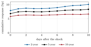
On the daily yield changes (in basis points), AIC keeps improving up to the ten lags it is allowed, and the VAR(10) is stable. The residuals have standard deviations of 7.9, 7.6 and 7.1 basis points and are strongly correlated (0.90 between the two- and five-year, 0.82 between the two- and ten-year, 0.94 between the five- and ten-year), so the ordering matters. With the two-year first, a one-standard-deviation two-year shock of 7.9 basis points moves the two-, five- and ten-year yields by a cumulative 10.1, 8.3 and 6.7 basis points over ten days (Figure 20.1), and it accounts for 67% of the ten-year’s ten-day forecast-error variance (the five-year’s shock for 21%, the ten-year’s own for 12%). The two-year leads, in this ordering, by construction; whether it leads in time is a separate question.

20.2 Causality in the predictive sense

Definition 20.4 (Granger causality)

A series $X$ Granger-causes $Y$ if the past of $X$ improves the prediction of $Y$ beyond the past of $Y$ and of the other variables (Granger, 1969); in a VAR, if the coefficients of the lags of $X$ in $Y$’s equation are not all zero, tested by an $F$-statistic.

It is predictive precedence, not causation: a common driver seen earlier in one series than in the other produces it, and so does a timing difference in how the data are recorded. On the daily yield changes, every pair Granger-causes the other at 5%, with $F(10, 12\,532)$ between 1.88 (two-year to ten-year, $p = 0.04$) and 7.16 (two-year to five-year, $p < 10^{-6}$); the ten-year to the two-year gives 2.83 ($p = 0.002$). With 12 574 days, tiny lead-lag effects are significant; none is large enough to trade on its own.

20.3 Cointegration and the error-correction form

Definition 20.5 (Cointegration, cointegrating vector, cointegration rank)

The components of a vector of unit-root processes are cointegrated (cointegration) if some linear combination $\beta^\top Y_t$ is stationary; $\beta$ is a cointegrating vector. The number of linearly independent cointegrating vectors is the cointegration rank $r$, and $k - r$ is the number of common stochastic trends.

Definition 20.6 (Vector error-correction model)

A vector error-correction model writes a VAR in differences plus a levels term, $\Delta Y_t = \alpha\beta^\top Y_{t-1} + \sum_{i=1}^{p-1}\Gamma_i\Delta Y_{t-i} + \mu + \varepsilon_t$, with $\alpha$ and $\beta$ of dimension $k \times r$: $\beta^\top Y_{t-1}$ is the deviation from equilibrium and $\alpha$ the speed at which each variable corrects it.

By the Granger representation theorem (Engle and Granger, 1987), a cointegrated system has an error-correction representation and conversely: a VAR in levels whose matrix $\Pi = \sum_iA_i - I$ has reduced rank $r$ factors as $\alpha\beta^\top$. A VAR in differences alone throws the levels information away; a VAR in levels keeps it but hides it. For the yields, $k = 3$; if their curve is driven by level and slope trends with a stationary curvature, $r = 1$ and the cointegrating vector is a fly.

Definition 20.7 (Engle–Granger test)

The Engle–Granger test regresses one variable on the others in levels and applies a Dickey–Fuller test to the residuals, with critical values that account for the estimated coefficients.

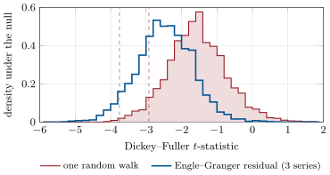
The least-squares residual is the most stationary-looking combination of the sample, so it looks stationary more often than a fixed one: its Dickey–Fuller statistic is shifted left, and the critical values depend on the number of variables. For three variables MacKinnon’s (2010) 5% value is $-3.74$, against $-2.86$ for one series; in the chapter’s simulation of 4 000 triples of independent random walks, using the one-series value would find cointegration 27% of the time (Figure 20.2). Regressing the five-year yield on the other two gives 0.40 times the two-year plus 0.62 times the ten-year, and a residual statistic of $-10.04$: cointegration, overwhelmingly.

20.4 Rank tests

Definition 20.8 (Johansen test)

The Johansen test (Johansen, 1988, 1991) estimates the VECM by maximum likelihood under the restriction $\operatorname{rank}\Pi = r$: after removing the short-run dynamics from $\Delta Y_t$ and $Y_{t-1}$, the squared canonical correlations $\hat\lambda_1 \ge \dots \ge \hat\lambda_k$ between the two residual sets give the trace statistic $-T\sum_{i>r}\ln(1 - \hat\lambda_i)$ for rank at most $r$, and the maximum-eigenvalue statistic $-T\ln(1 - \hat\lambda_{r+1})$; the corresponding eigenvectors estimate $\beta$.

The null distributions are functionals of Brownian motion that depend on the number of common trends and on the deterministic terms. With the constant restricted to the cointegrating space (yields have no trend), the chapter simulates them from 20 000 systems of random walks of 2 000 days; the 95% points of the trace statistic are 35.23, 20.36 and 9.23 for three, two and one common trend.

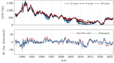
On the three yields, 1976–2026, with nine lagged differences (the VAR(10) of AIC), the trace statistics are 59.77 for rank zero, 14.93 for rank at most one and 2.34 for rank at most two: rank one, a single cointegrating vector. Normalised on the five-year yield, it is $0.41 \times$ two-year $- 1 \times$ five-year $+ 0.61 \times$ ten-year: a fly whose wings sum to 1.02, close to level-neutral, but tilted toward the ten-year, so that it also neutralises most of the slope. As an AR(1), it reverts with coefficient 0.9841, a half-life of 43 trading days; the one-two-one fly (scaled to the same five-year weight) has coefficient 0.9891 and a half-life of 63 days, and a daily volatility of 2.15 basis points against 2.06 (Figure 20.3).

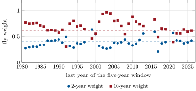
The weights are an estimate, and not a stable one. On five-year rolling windows, the trace test finds no cointegration at 5% in 20 of the 46 windows, and in the windows where it finds one vector, the two-year weight ranges from 0.27 to 0.63 and the ten-year weight from 0.40 to 0.97 (Figure 20.4). Fifty years pin the fly down; five years do not, and a desk that trades the fly lives in the five years.

20.5 Tutorial: the fly that mean-reverts

20.6 Build: the cointegration module

20.7 Exercises

Exercise 20.1 ★

Is the VAR(1) with $A = \left(\begin{smallmatrix}0.5 & 0.4\\ 0.4 & 0.5\end{smallmatrix}\right)$ stationary? And with $\left(\begin{smallmatrix}0.6 & 0.4\\ 0.4 & 0.6\end{smallmatrix}\right)$?

Solution

Solution of Exercise 20.1.

The eigenvalues of the first matrix are $0.9$ and $0.1$: stationary. Those of the second are $1.0$ and $0.2$: a unit root, so not stationary; the sum $x + y$ follows a random walk while the difference $x - y$ is stationary (with coefficient 0.2): the two series are cointegrated with $\beta = (1, -1)$.

Exercise 20.2 ★

Two yields $x$ and $y$ are random walks with $y - 0.9x$ stationary. What are $k$, $r$ and the number of common trends?

Solution

Solution of Exercise 20.2.

$k = 2$, $r = 1$ (the vector $(1, -0.9)$ up to scale), and $k - r = 1$ common trend.

Exercise 20.3 ★

Compute MacKinnon’s 5% Engle–Granger critical value for three variables and $T = 500$ from $(-3.74066, -8.5631, -10.852, 27.982)$.

Solution

Solution of Exercise 20.3.

$-3.74066 - 8.5631/500 - 10.852/500^2 + 27.982/500^3 = -3.758$.

Exercise 20.4 ★★

Write the VECM of $y_t = 0.9x_{t-1} + 0.5(y_{t-1} - 0.9x_{t-1}) + e_t$ with $x$ a random walk, and identify $\alpha$ and $\beta$.

Solution

Solution of Exercise 20.4.

$\Delta y_t = -0.5(y_{t-1} - 0.9x_{t-1}) + e_t$ and $\Delta x_t = u_t$. So $\beta = (1, -0.9)^\top$ and $\alpha = (-0.5, 0)^\top$ for $(y, x)$: $y$ corrects half of any deviation each period; $x$ does not correct at all (it is weakly exogenous).

Exercise 20.5 ★★

Two residuals have correlation 0.9 and unit variances. With the first variable ordered first, what fraction of the second variable’s one-step forecast variance is attributed to the first shock?

Solution

Solution of Exercise 20.5.

The Cholesky factor writes the second residual as $0.9z_1 + \sqrt{0.19}\,z_2$, so 81% of its one-step variance is attributed to the first shock; with the opposite ordering it would be 19% (or 0% of the first variable’s to the second shock in the original ordering).

Exercise 20.6 ★★

The Johansen eigenvalues of a three-variable system with $T = 1\,000$ are 0.05, 0.01 and 0.002. Compute the trace statistics and the rank at 5%.

Solution

Solution of Exercise 20.6.

Trace for $r = 0$: $-1\,000(\ln0.95 + \ln0.99 + \ln0.998) = 63.35$; $r \le 1$: 12.05; $r \le 2$: 2.00. Against 35.23, 20.36 and 9.23: reject $r = 0$, not $r \le 1$, so rank one.

Exercise 20.7 ★★★

Coding. Estimate the Johansen fly weights on rolling five-year windows of the yields, and count the windows in which the trace test finds no cointegration.

Solution

Solution of Exercise 20.7.

rolling_weights(): no cointegration at 5% in 20 of the 46 windows; where one vector is found, the 2-year weight ranges from 0.27 to 0.63 and the 10-year weight from 0.40 to 0.97.

Exercise 20.8 ★★★

Find the flaw. “We regressed the 5-year yield on the 2-year and 10-year, got a residual whose Dickey–Fuller statistic is $-3.1$, below the 5% critical value of $-2.86$, and started trading the residual as a stationary fly.”

Solution

Solution of Exercise 20.8.

The residual of an estimated regression must be judged with Engle–Granger critical values, $-3.74$ at 5% for three variables, not $-2.86$; $-3.1$ does not reject the null of no cointegration. With the Dickey–Fuller value, independent random walks would pass 27% of the time. The weights should also be checked for stability before the fly is traded.

20.8 Problem: The Fly That Mean-Reverts

Problem 20.1

Weekend problem — the cointegrating 2s5s10s fly

The data are the daily 2-, 5- and 10-year constant-maturity Treasury yields (FRED DGS2, DGS5, DGS10), 1 June 1976 to 22 September 2026, 12 574 days, in basis points.

Part I — Each series.

1. What do Dickey–Fuller tests say about each yield?
2. What VAR order does AIC choose for the daily changes, and is the VAR stable?
3. What are the residual standard deviations and correlations?
4. What does a one-standard-deviation 2-year shock do over ten days?
5. Which yields Granger-cause which, and what does it mean?

Part II — Cointegration.

6. What are the Johansen trace statistics and the rank at 5%?
7. What are the fly weights per unit of the 5-year, and what do they neutralise?
8. What does Engle–Granger give, against which critical value?
9. What are the half-lives of the Johansen fly and of the one-two-one fly?
10. What are the flies’ daily volatilities?

Part III — Robustness.

11. How often does a five-year window find cointegration?
12. How much do the weights move across windows?
13. Why is the Engle–Granger critical value lower than Dickey–Fuller’s?
14. How would you correct the half-life for the small-sample bias of chapter 17?
15. What would a desk risk by trading the full-sample weights?

Part IV — Judgement.

16. Which fly would you trade, with which weights?
17. How would you size it for a half-life of 43 days?
18. Why should the weights be re-estimated, and how often?
19. State the named result: the Johansen fly weights and half-life against the one-two-one fly’s.
20. In one sentence: what does cointegration promise a relative-value trader, and what not?

Solution

Solution of Problem 20.1.

1. Dickey–Fuller statistics $-1.30$, $-1.33$, $-1.31$: no yield rejects a unit root. 2. AIC keeps improving up to the maximum of ten lags; the VAR(10) of the changes is stable. 3. 7.9, 7.6 and 7.1 bp; correlations 0.90 (2y–5y), 0.82 (2y–10y), 0.94 (5y–10y). 4. With the 2-year ordered first, a 7.9 bp shock moves the 2-, 5- and 10-year yields by 10.1, 8.3 and 6.7 bp cumulatively over ten days, and explains 67% of the 10-year’s ten-day forecast-error variance. 5. All six directions are significant at 5% ($F$ from 1.88 to 7.16 with 10 and 12 532 degrees of freedom): with so much data, small lead-lag effects from timing and common news are detectable; they are predictive precedence, not causation. 6. 59.77, 14.93 and 2.34 against 35.23, 20.36 and 9.23: rank one. 7. $0.41 \times$ 2-year $- 1 \times$ 5-year $+ 0.61 \times$ 10-year: the wings sum to 1.02 (level-neutral), and the tilt toward the 10-year also neutralises most of the slope. 8. The 5-year on the others: $0.40$ and $0.62$, residual statistic $-10.04$ against a 5% critical value of $-3.74$. 9. 43 trading days (AR coefficient 0.9841) against 63 (0.9891). 10. 2.06 and 2.15 bp a day (the one-two-one fly scaled to the same 5-year weight). 11. In 26 of 46 windows (20 find none at 5%). 12. The 2-year weight from 0.27 to 0.63 and the 10-year from 0.40 to 0.97, among the windows that find one vector. 13. Least squares chooses the combination that looks most stationary in the sample, so the residual’s statistic is pushed left even when nothing is cointegrated; the more variables, the further. 14. Apply Kendall’s correction $(1 + 3\hat\rho)/n$ to the fly’s AR(1) coefficient: 0.9841 becomes 0.9844 with 12 574 days and the half-life 44 days instead of 43; then simulate its distribution as in chapter 17. 15. That the weights of the next years differ, so the traded fly carries level or slope exposure it was meant to remove, and reverts more slowly than the backtest promised. 16. The Johansen fly, with weights re-estimated on a recent window and bounded near the long-run values, cross-checked against duration-neutral weights. 17. By the fly’s stationary standard deviation, $2.06/\sqrt{1 - 0.9841^2} = 11.6$ bp: size so that a two- or three-standard-deviation move (25 to 35 bp) is survivable, and expect a typical deviation to halve in about two months. 18. Because the curve’s factor loadings change with the rate regime; re-estimate on a rolling window every month or quarter and trade only when the rank test still finds the vector. 19. Named result: the fly that mean-reverts: the Johansen cointegrating fly of the 2-, 5- and 10-year yields, 1976–2026, weights the wings $0.41$ and $0.61$ per unit of the 5-year and reverts with a half-life of 43 trading days, against 63 for the one-two-one fly. 20. It promises that a basket’s deviations are temporary on average; it does not promise how long they last, how large they get first, or that the weights will stay the same.

20.9 Interview questions

Interview question 20.1 ★ researcher, trader

What is the difference between correlation and cointegration?

Solution

Solution of Interview question 20.1.

Correlation describes co-movement of changes over a horizon; cointegration says that the levels share stochastic trends, so some combination of them is stationary. Two series can be highly correlated and drift apart forever, or weakly correlated day to day and tied together in the long run.

What the interviewer is looking for: Changes versus levels, and a counterexample either way.

Interview question 20.2 ★★ researcher, trader

How would you choose the weights of a curve fly to trade mean reversion?

Solution

Solution of Interview question 20.2.

Choose weights that make the fly stationary and fast-reverting: estimate the cointegrating vector (Johansen or Engle–Granger with the right critical values), compare with duration- or PCA-neutral weights, check stability on rolling windows, and measure the half-life and volatility of the resulting fly.

What the interviewer is looking for: Stationarity as the criterion, the right test, and stability.

Interview question 20.3 ★★ researcher

Why can’t you use the Dickey–Fuller critical values on the residual of a cointegrating regression?

Solution

Solution of Interview question 20.3.

The coefficients were estimated to make the residual as small, and so as stationary-looking, as possible; under the null the residual’s statistic is shifted left, and the shift grows with the number of regressors. Use Engle–Granger (MacKinnon) critical values: $-3.34$ for two variables, $-3.74$ for three at 5%, asymptotically.

What the interviewer is looking for: The pre-fitting argument and the right table.

Interview question 20.4 ★★ researcher, mle

What does Granger causality test, and what does it not?

Solution

Solution of Interview question 20.4.

Whether the past of one series improves forecasts of another given its own past; it tests predictive precedence within the information set used. It does not establish causation: omitted common drivers, timing differences in data, and expectations can all produce it.

What the interviewer is looking for: Prediction, not causation, and the omitted-variable caveat.

Interview question 20.5 ★★ researcher

Why does the ordering matter in a VAR’s impulse responses?

Solution

Solution of Interview question 20.5.

Because correlated shocks are split by a Cholesky factorisation: the first variable gets all the common part of the shock. Different orderings attribute the contemporaneous correlation differently; report the ordering, try alternatives, or use generalised responses.

What the interviewer is looking for: Orthogonalisation and its arbitrariness.

Interview question 20.6 ★★★ researcher

Explain the Johansen test in terms of canonical correlations.

Solution

Solution of Interview question 20.6.

After partialling out the short-run lags, compute the canonical correlations between the differences $\Delta Y_t$ and the lagged levels $Y_{t-1}$. Stationary combinations of the levels predict the differences, so they have large canonical correlations; the number of significantly nonzero ones is the rank, the eigenvectors estimate $\beta$, and the trace statistic sums $-T\ln(1 - \lambda_i)$ over the smallest ones.

What the interviewer is looking for: Reduced-rank regression through canonical correlations.