Quantitative Methods · Methods

25Floating Point and Numerical Linear Algebra

In January 1982 the Vancouver Stock Exchange launched an index at 1000. It was recomputed after every trade, a few thousand times a day, and after each recomputation it was truncated to three decimals, not rounded. Twenty-two months later, on Friday 25 November 1983, it closed at 524.811 in a market that had in fact risen; recomputed over that weekend, it stood at 1098.892. Each truncation cost less than a thousandth of a point. A million of them cost half the index. This chapter is about what the machine does with numbers: the format of a floating-point number and the rounding of every operation, cancellation and the accumulation of error, the condition of a problem and the stability of an algorithm, the factorisations that numerical linear algebra is built on, iterative solvers, and the reproducibility that a risk system owes its users.

25.1 Representation

Definition 25.1 (Floating-point number, machine epsilon, unit in the last place)

A binary floating-point number is $\pm m \times 2^e$ with an integer significand $m$ of $p$ bits and an exponent $e$ in a fixed range; IEEE 754 double precision (binary64) has $p = 53$ and exponents from $-1022$ to $1023$ . Machine epsilon is the gap between 1 and the next larger number, $2^{1-p} = 2^{-52} \approx 2.2 \times 10^{-16}$ ; the unit roundoff $u$ is half of it (some texts, and some libraries, call $u$ itself machine epsilon). A unit in the last place (ulp) of $x$ is the gap between the two floating-point numbers around $x$ .

Definition 25.2 (Subnormal number, fused multiply-add)

A subnormal number fills the gap between zero and the smallest normal number with a reduced significand, so that $x - y = 0$ only if $x = y$ . A fused multiply-add computes $a \times b + c$ with a single rounding.

The standard model of arithmetic: every basic operation returns the exact result rounded, $\mathrm{fl}(x \circ y) = (x \circ y)(1 + \delta)$ with $|\delta| \le u = 2^{-53}$ . Most decimal fractions are not representable: $0.1$ is stored as the nearest binary64 number, a little above $0.1$ , so $0.1 \times 10 - 1$ evaluates to exactly 0 with two roundings, while a fused multiply-add, rounding once, returns $2^{-54}$ . Both are correct IEEE results. A compiler that contracts $a \times b + c$ into a fused multiply-add changes the answer: GCC does so by default outside a standards-compliant C mode (-ffp-contract=fast) when the target has the instruction, which is one reason a C++ and a Python risk engine can disagree in the last bits.

25.2 Cancellation and the accumulation of error

Definition 25.3 (Catastrophic cancellation, compensated summation, Welford’s algorithm)

Catastrophic cancellation is the loss of relative accuracy when two nearly equal rounded numbers are subtracted: the leading digits cancel and the rounding errors remain. Compensated summation (Kahan, 1965; in Neumaier’s variant, 1974) carries the rounding error of each addition in a separate variable and adds it back. Welford’s algorithm (1962) updates a running mean and sum of squared deviations one observation at a time.

Proposition 25.4 (Summation error bounds)

Recursive summation of $n$ numbers has error at most $(n - 1)u\sum_i|x_i| + O(u^2)$ ; pairwise summation at most $\lceil\log_2n\rceil u\sum_i|x_i| + O(u^2)$ ; compensated summation at most $2u\sum_i|x_i| + O(nu^2)\sum_i|x_i|$ , independent of $n$ to first order.

Proof. In recursive summation the partial sum $s_k$ is rounded once per step, so $x_1$ passes through $n - 1$ roundings, each contributing a relative error at most $u$ of a partial sum bounded by $\sum|x_i|$ ; pairwise summation passes each term through only $\lceil\log_2n\rceil$ additions. In compensated summation the error of each addition is computed exactly (for $|s| \ge |x|$ , $(s - t) + x$ is exact) and fed back, so only the final correction and second-order terms remain. ∎

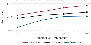
On a million P&L entries spanning seven orders of magnitude, the error against the exact rational sum is $2.5 \times 10^{-6}$ for the naive loop, $2.8 \times 10^{-8}$ for pairwise summation and $2.2 \times 10^{-9}$ , less than one unit in the last place of the total ( $7.5 \times 10^{-9}$ ), for Neumaier’s (Figure 25.1). None matters for a P&L report; all matter when two systems must agree to the cent and one of them sums in a different order.

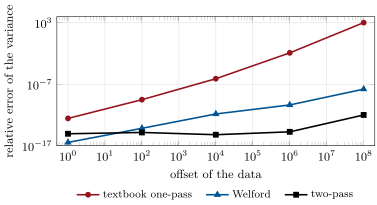
Error of three summation algorithms against the exact (rational) sum of n simulated P&L entries whose magnitudes cycle over seven orders. Neumaier’s compensated sum stays below one unit in the last place of the total. Data: the chapter’s tutorial, seeded. — **Figure 25.1.** Error of three summation algorithms against the exact (rational) sum of $n$ simulated P&L entries whose magnitudes cycle over seven orders. Neumaier’s compensated sum stays below one unit in the last place of the total. Data: the chapter’s tutorial, seeded.

The textbook variance, $(\sum x_i^2 - (\sum x_i)^2/n)/(n - 1)$ , subtracts two nearly equal large numbers. On ten thousand prices equal to an offset plus a uniform draw, its relative error is $3 \times 10^{-13}$ with offset 1, $8.0 \times 10^{-7}$ with offset $10^4$ (prices near 10 000), 1.3% with offset $10^6$ , and with offset $10^8$ it returns 86.8 for a true variance of 0.082. The two-pass formula, which subtracts the mean first, stays near $10^{-12}$ or below; Welford’s update within $1.6 \times 10^{-8}$ even at $10^8$ (Figure 25.2).

Relative error of three variance formulas on 10 000 values equal to an offset plus a uniform draw on (0, 1) (true variance 0.082), against the exact rational result. The one-pass textbook formula loses all accuracy as the offset grows. Data: the chapter’s tutorial, seeded. — **Figure 25.2.** Relative error of three variance formulas on 10 000 values equal to an offset plus a uniform draw on $(0, 1)$ (true variance 0.082), against the exact rational result. The one-pass textbook formula loses all accuracy as the offset grows. Data: the chapter’s tutorial, seeded.

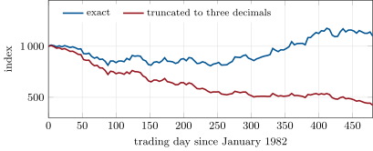
The Vancouver index is the same mechanism with a bias. Rounding to three decimals makes errors of either sign that average out; truncating removes, on average, half a thousandth at each recalculation, always downward. At 2 400 recalculations a day over 480 trading days the expected loss is $0.0005 \times 1\,152\,000 = 576$ points, against a documented shortfall of $1098.892 - 524.811 = 574$ ; at the “about 3 000” a day sometimes quoted it would be 720. A simulation of the recalculations, with an exact index rising to 1098.9, ends at 422 when truncated (the drift compounds with the index’s own moves) and at 1098.57 when rounded (Figure 25.3).

**Figure 25.3.** A simulated index recomputed 2 400 times a day for 480 trading days, exactly and with truncation to three decimals after each recomputation; the exact index is set to end at the corrected Vancouver value of 1098.892. Data: the chapter’s tutorial, seeded.

25.3 Conditioning and stability

Definition 25.5 (Condition number, backward error, backward stability)

The condition number of a problem bounds the relative change of its answer per relative change of its data; for solving $Ax = b$ it is $\kappa(A) = \lVert A\rVert\lVert A^{-1}\rVert$ , the ratio of extreme singular values in the 2-norm. The backward error of a computed answer is the smallest perturbation of the data for which it is exact. An algorithm has backward stability if its backward error is always of the order of the unit roundoff.

Proposition 25.6 (Forward error, condition and backward error)

If $\hat x$ solves $(A + \Delta A)\hat x = b$ with $\lVert\Delta A\rVert/\lVert A\rVert = \epsilon$ and $\kappa(A)\epsilon < 1$ , then $\lVert\hat x - x\rVert/\lVert x\rVert \le \kappa(A)\epsilon/(1 - \kappa(A)\epsilon)$ : to first order, forward error is at most condition number times backward error.

Proof. Subtracting $Ax = b$ gives $A(\hat x - x) = -\Delta A\,\hat x$ , so $\lVert\hat x - x\rVert \le \lVert A^{-1}\rVert\lVert\Delta A\rVert\lVert\hat x\rVert = \kappa\epsilon\lVert\hat x\rVert$ , and $\lVert\hat x\rVert \le \lVert x\rVert + \lVert\hat x - x\rVert$ gives the bound. ∎

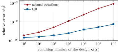
A backward-stable algorithm on a problem with condition number $10^8$ can lose eight of its sixteen digits, and no algorithm can do better, because the data are only known to rounding. What an algorithm can do is not make the conditioning worse. The normal equations of least squares, $X^\top X\beta = X^\top y$ , solve a problem whose condition number is $\kappa(X)^2$ ; a QR factorisation of $X$ solves one with $\kappa(X)$ . On five regressors with condition number $10^7$ , the normal equations lose all but two digits of the coefficients (relative error $5 \times 10^{-3}$ ), the QR solution keeps about ten (an error near $10^{-10}$ , whose exact digits are rounding and move with the linear-algebra library and the processor) (Figure 25.4). That is chapter 16’s multicollinearity seen from the machine’s side.

Least squares on an exactly consistent system of 500 observations and five regressors whose design has condition number : relative error of the coefficients from the normal equations (which square ) and from a QR factorisation. Data: the chapter’s tutorial, seeded. — **Figure 25.4.** Least squares on an exactly consistent system of 500 observations and five regressors whose design has condition number $\kappa$ : relative error of the coefficients from the normal equations (which square $\kappa$ ) and from a QR factorisation. Data: the chapter’s tutorial, seeded.

25.4 Factorisations

Definition 25.7 (LU, Cholesky, QR and singular value decompositions)

The LU factorisation writes $PA = LU$ with a permutation $P$ (partial pivoting), unit lower-triangular $L$ and upper-triangular $U$ . The Cholesky factorisation of a symmetric positive-definite matrix is $A = LL^\top$ with $L$ lower triangular. The QR factorisation writes $A = QR$ with orthonormal columns in $Q$ and $R$ upper triangular. The singular value decomposition writes $A = U\Sigma V^\top$ with orthonormal $U$ , $V$ and a nonnegative diagonal $\Sigma$ . The tridiagonal matrix algorithm (Thomas’s algorithm) solves a tridiagonal system by one forward elimination and one back substitution, in $O(n)$ operations.

Proposition 25.8 (Cholesky succeeds exactly for positive-definite matrices)

The Cholesky recursion $\ell_{jj} = (a_{jj} - \sum_{k<j}\ell_{jk}^2)^{1/2}$ , $\ell_{ij} = (a_{ij} - \sum_{k<j}\ell_{ik}\ell_{jk})/\ell_{jj}$ finds a positive pivot at every step if and only if $A$ is symmetric positive definite.

Proof. The $j$ -th pivot is the ratio of the leading principal minors of orders $j$ and $j - 1$ , so every pivot is positive if and only if every leading minor is, which (Sylvester) is positive definiteness. ∎

A failed Cholesky is therefore a test, and a useful one: the pairwise correlation matrix of chapter 23 (fifty series, half the data missing) fails at the sixth pivot, which is $-0.14$ . Adding a multiple of the identity (“jitter”) cannot succeed until the multiple exceeds the magnitude of the most negative eigenvalue, 1.42, more than the unit diagonal itself, which destroys the correlations; the nearest correlation matrix of chapter 23 passes with a jitter of $10^{-8}$ . Each factorisation has its use: LU for general systems, Cholesky for covariances (and to simulate correlated normals), QR for least squares, the SVD for rank and conditioning, and Thomas’s algorithm for the finite-difference grids of chapter 27.

25.5 Iterative solvers

Definition 25.9 (Conjugate gradient method, preconditioner)

The conjugate gradient method (Hestenes and Stiefel, 1952) solves $Ax = b$ for symmetric positive-definite $A$ by minimising $\frac12x^\top Ax - b^\top x$ along mutually $A$ -conjugate directions built from the residuals. A preconditioner $M \approx A$ replaces the system by one with $M^{-1}A$ , of smaller condition number.

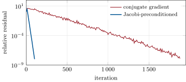
In exact arithmetic conjugate gradient terminates in at most $n$ steps, and the error after $k$ steps falls at least like $2\bigl((\sqrt\kappa - 1)/(\sqrt\kappa + 1)\bigr)^k$ . In floating point the directions lose conjugacy and the finite termination is lost, but the rate survives. On a 400-dimensional system with condition number $1.1 \times 10^5$ , whose rows and columns are badly scaled, conjugate gradient needs about 1 900 iterations to reduce the residual by $10^8$ , almost five times $n$ (the exact count moves by a few dozen with the order in which the linear-algebra library sums, one thread or four: the lost conjugacy is rounding, and rounding depends on that order); with a Jacobi (diagonal) preconditioner, which brings the condition number to about 100, it needs 102 (Figure 25.5).

Conjugate gradient on a badly scaled symmetric positive-definite system of dimension 400 (condition number 1.1 × 105), with and without a diagonal preconditioner: relative residual against the iteration (the preconditioned run stops at 102). Data: the chapter’s tutorial, seeded. — **Figure 25.5.** Conjugate gradient on a badly scaled symmetric positive-definite system of dimension 400 (condition number $1.1 \times 10^5$ ), with and without a diagonal preconditioner: relative residual against the iteration (the preconditioned run stops at 102). Data: the chapter’s tutorial, seeded.

25.6 The bugs that cost money

Definition 25.10 (Reproducibility to the bit)

A computation has bitwise reproducibility if the same inputs give the same bits on every run, machine, compiler and language used to compute them.

Floating-point addition is not associative, so anything that changes the order of operations changes the last bits: a parallel reduction with a different thread count, a vectorised loop, a compiler that contracts to fused multiply-adds, a library that sums in blocks. Those bits then propagate through thresholds (a limit breached or not, a trade filled or not) and become real differences. The firm’s kit therefore fixes the order of every operation: its three twins, in Python, C++20 and Rust, perform the same operations in the same order on the same SplitMix64 inputs and agree bit for bit on the naive, pairwise and compensated sums of ten thousand P&L entries, Welford’s mean and variance of ten thousand prices, a log-sum-exp and a tridiagonal solve; a test in each language asserts the same 64-bit patterns. The same test with a fused multiply-add in place of a multiply and an add shows the difference: $0.1 \times 10 - 1$ is 0 one way and $2^{-54}$ the other. (With g++ -std=c++20 -O2 on x86-64 no contraction happens, because the baseline instruction set has no fused multiply-add; -march=native on a recent processor turns it on.)

The Vancouver mechanism, a systematic rounding repeated millions of times, has cost more than money. On 25 February 1991 a Patriot air-defence battery at Dhahran, Saudi Arabia, failed to intercept a Scud missile, which hit an Army barracks and killed 28 Americans. The General Accounting Office traced the failure to the system clock: time was counted in tenths of a second and multiplied by $\frac1{10}$ in 24-bit registers, and after the battery had run for about 100 hours the computed time was 0.3433 seconds off, enough to shift the tracking window by 687 metres. The report’s figures are what $\frac1{10}$ chopped to 23 binary places gives: it is short by $9.5 \times 10^{-8}$ , and $3\,600\,000$ tenths of a second accumulate $0.3433$ seconds. Israeli data had shown the loss of accuracy after eight hours; the corrected software arrived the day after the attack.

Not every numerical bug is in the last bit. The management task force that reviewed JPMorgan Chase’s 2012 Chief Investment Office losses reported, among the errors found in a new value-at-risk model run in spreadsheets, that “after subtracting the old rate from the new rate, the spreadsheet divided by their sum instead of their average”, which “likely had the effect of muting volatility by a factor of two and of lowering the VaR”. The defence is the same as for rounding: an independent implementation, reference results asserted in tests, and a reviewer who recomputes one number by hand.

25.7 Tutorial: the index that lost half its value

Goal. Reproduce the Vancouver drift, measure summation and variance errors against exact arithmetic, watch Cholesky fail, and check that three languages agree bit for bit. End state: Figures 25.1, 25.2 and 25.3 and the bit patterns of reference_results() in the three test suites.

Compensated summation and Welford’s update in Python.

def neumaier_sum(x) -> float:
    """Kahan's compensated summation in Neumaier's form: the rounding error of each addition is carried in c."""
    s, c = 0.0, 0.0
    for v in x:
        v = float(v)
        t = s + v
        if abs(s) >= abs(v):
            c += (s - t) + v
        else:
            c += (v - t) + s
        s = t
    return s + c


def welford(x) -> tuple[int, float, float]:
    n, mean, m2 = 0, 0.0, 0.0
    for v in x:
        v = float(v)
        n += 1
        d = v - mean
        mean += d / n
        m2 += d * (v - mean)
    return n, mean, (m2 / (n - 1) if n > 1 else math.nan)

Listing 25.1. Neumaier summation and Welford’s algorithm (Python). code/firm/fpkit/firm_fpkit.py

The same operations in Rust, in the same order.

pub fn neumaier_sum(x: &[f64]) -> f64 {
    let (mut s, mut c) = (0.0f64, 0.0f64);
    for &v in x {
        let t = s + v;
        if s.abs() >= v.abs() {
            c += (s - t) + v;
        } else {
            c += (v - t) + s;
        }
        s = t;
    }
    s + c
}

/// (n, mean, variance with divisor n - 1)
pub fn welford(x: &[f64]) -> (usize, f64, f64) {
    let (mut n, mut mean, mut m2) = (0usize, 0.0f64, 0.0f64);
    for &v in x {
        n += 1;
        let d = v - mean;
        mean += d / n as f64;
        m2 += d * (v - mean);
    }
    (n, mean, if n > 1 { m2 / (n - 1) as f64 } else { f64::NAN })
}

Listing 25.2. Neumaier summation and Welford’s algorithm (Rust twin). code/firm/fpkit/rust/src/lib.rs

Run vancouver(), summation_errors(), variance_errors(), normal_equations(), cholesky_on_pairwise() and cg_demo() in qm_float.py; then the three test suites of firm.fpkit, and fig_float.py.

What to change next. Compile the C++ twin with -march=native -ffp-contract=fast and see which asserted bit patterns break; sum the P&L with NumPy’s sum and explain why it is closer to pairwise than to naive.

25.8 Build: the numerics kit

Purpose. Numerically careful primitives, identical in the three languages of the miniature firm, so that a risk number computed in the research notebook, the C++ engine and the Rust gateway is the same number.

Interface. SplitMix64; naive_sum, pairwise_sum, neumaier_sum; welford, welford_cov; logsumexp; thomas; in Python also cholesky(A, jitter), cg(A, b, precond), fma_exact, bits.

Rules. No fast-math, no floating-point contraction in the builds that must reproduce; fixed summation order; every twin asserts the reference bit patterns; a failed Cholesky is reported with its index, never silently jittered.

Acceptance tests. code/firm/fpkit/tests/, cpp/firm_fpkit_test.cpp, rust/src/lib.rs: identical bits across the three languages; Neumaier equals the exact sum here; Welford against exact rational arithmetic; Thomas against a dense solve; Cholesky on positive-definite and indefinite matrices; conjugate gradient; the fused multiply-add example.

Stretch. A reproducible parallel sum (fixed blocking plus compensation); double-double arithmetic; a pivoted Cholesky that returns the rank.

Sources and further reading

IEEE Standard for Floating-Point Arithmetic, IEEE Std 754-2019.
W. Kahan, “Further remarks on reducing truncation errors”, Communications of the ACM 8, 1965; A. Neumaier, Zeitschrift für Angewandte Mathematik und Mechanik 54, 1974.
B. P. Welford, “Note on a method for calculating corrected sums of squares and products”, Technometrics 4, 1962.
M. R. Hestenes and E. Stiefel, “Methods of conjugate gradients for solving linear systems”, Journal of Research of the National Bureau of Standards 49, 1952.
N. J. Higham, Accuracy and Stability of Numerical Algorithms, 2nd ed., SIAM, 2002.
D. Goldberg, “What every computer scientist should know about floating-point arithmetic”, ACM Computing Surveys 23, 1991.
GCC manual, “Options that control optimization” (-ffp-contract), accessed 24 September 2026.
US General Accounting Office, Patriot Missile Defense: Software Problem Led to System Failure at Dhahran, Saudi Arabia, GAO/IMTEC-92-26, 4 February 1992.
On the Vancouver index: K. Quinn, The Wall Street Journal, 8 November 1983, p. 37, and W. Lilley, The Toronto Star, 29 November 1983, p. 35, as cited in the Wikipedia article “Vancouver Stock Exchange” (accessed 24 September 2026).

25.9 Exercises

Exercise 25.1 ★

What are the unit roundoff and machine epsilon of binary64, and how many significant decimal digits does it carry?

Solution

Solution of Exercise 25.1.

Unit roundoff $u = 2^{-53} \approx 1.11 \times 10^{-16}$ , machine epsilon $2^{-52} \approx 2.22 \times 10^{-16}$ ; $53\log_{10}2 \approx 15.95$ , so fifteen to sixteen significant decimal digits.

Exercise 25.2 ★

An index is truncated to two decimals after each of 10 000 daily recalculations. What drift should one expect in a year of 250 days?

Solution

Solution of Exercise 25.2.

Half a hundredth per recalculation: $0.005 \times 10\,000 \times 250 = 12\,500$ points a year, downward, before the compounding with the index’s own moves.

Exercise 25.3 ★

Why is $10^8 + 1 - 10^8$ exact in double precision, but $10^{16} + 1 - 10^{16}$ not?

Solution

Solution of Exercise 25.3.

$10^8 + 1$ needs 27 bits and is representable, so both operations are exact. Above $2^{53} \approx 9.0 \times 10^{15}$ the spacing of doubles is 2, so $10^{16} + 1$ is a tie, rounded to the neighbour with an even significand, which is $10^{16}$ : the result is 0.

Exercise 25.4 ★★

Show that the textbook variance formula’s absolute error is of order $u\sum x_i^2/(n - 1)$ , and estimate the relative error for prices near 10 000 with variance 0.08.

Solution

Solution of Exercise 25.4.

Each of $\sum x_i^2$ and $(\sum x_i)^2/n$ is about $nc^2$ and carries a rounding error of at least $u\,nc^2$ (more with recursive summation); their difference, divided by $n - 1$ , has an absolute error of order $uc^2$ . With $c = 10^4$ : $1.1 \times 10^{-16} \times 10^8 \approx 10^{-8}$ , or about $10^{-7}$ relative to a variance of 0.08; the summation error pushes it up, and the tutorial measures $8.0 \times 10^{-7}$ .

Exercise 25.5 ★★

A design matrix has condition number $10^5$ . How many digits can the normal equations lose, and QR?

Solution

Solution of Exercise 25.5.

The normal equations work with $\kappa^2 = 10^{10}$ and can lose about ten of sixteen digits; QR, with $\kappa = 10^5$ , about five.

Exercise 25.6 ★★

Show that the log-sum-exp trick, $m + \log\sum e^{x_i - m}$ with $m = \max x_i$ , never overflows, and compute $\log(e^{1000} + e^{1000})$ .

Solution

Solution of Exercise 25.6.

All the $x_i - m$ are at most 0, so each exponential is at most 1 and the largest is exactly 1: the sum lies in $[1, n]$ and its logarithm cannot overflow or be $-\infty$ . $\log(e^{1000} + e^{1000}) = 1000 + \ln2 = 1000.693$ , where the direct formula overflows to infinity.

Exercise 25.7 ★★★

Coding. Sum a million simulated P&L entries naively, pairwise and with Neumaier’s compensation, and compare with the exact rational sum.

Solution

Solution of Exercise 25.7.

summation_errors(): at $n = 10^6$ the errors against the exact rational sum (47 878 411.409) are $2.5 \times 10^{-6}$ (naive), $2.8 \times 10^{-8}$ (pairwise) and $2.2 \times 10^{-9}$ (Neumaier), the last below one unit in the last place ( $7.5 \times 10^{-9}$ ).

Exercise 25.8 ★★★

Find the flaw. “Our risk totals differ between the C++ engine and the Python reports in the tenth significant digit, so one of the two has a bug.”

Solution

Solution of Exercise 25.8.

A difference in the tenth digit is what different operation orders, fused multiply-add contraction or different exp and log implementations produce on a moderately conditioned computation; it is not evidence of a bug. Evidence would be a difference larger than the condition number times the unit roundoff, or a difference on reference inputs where both engines are meant to perform identical operations. Either fix the order and flags and assert bits, or compare with a tolerance justified by the conditioning.

25.10 Problem: The Index That Lost Half Its Value

Problem 25.1

Weekend problem — truncation, a million times

An index starts at 1000 and is recomputed after every trade, 2 400 times a day for 480 trading days; after each recomputation it is truncated to three decimals. The documented case: 524.811 before the correction, 1098.892 after.

Part I — The drift.

What is the expected loss from one truncation, and why?
What is the expected total loss, and how does it compare with the documented shortfall?
What would it be at 3 000 recalculations a day?
What does rounding instead of truncating change?
Where does the simulated truncated index end, and why lower than the formula?

Part II — Accumulated error.

How large are the naive, pairwise and compensated summation errors on a million P&L entries?
How wrong is the textbook variance for prices near 10 000, $10^6$ and $10^8$ ?
Why do the two-pass and Welford formulas survive?
How many digits do the normal equations lose at condition number $10^7$ , and QR?
Where and why does the Cholesky factorisation of the pairwise correlation matrix fail?

Part III — Reproducibility.

What do the three language twins agree on, and how is it checked?
What does a fused multiply-add change in $0.1 \times 10 - 1$ ?
Which compiler setting can silently introduce fused multiply-adds?
How many conjugate-gradient iterations does the badly scaled system need, with and without the Jacobi preconditioner?
Why does conjugate gradient not stop after $n$ steps here?

Part IV — Judgement.

How would you have caught the Vancouver error within a week?
What should a risk system log so that two runs can be compared bit for bit?
When is bitwise reproducibility worth its cost?
State the named result: the expected drift per recalculation times the number of recalculations against the documented shortfall.
In one sentence: what does the machine do to every number you compute?

Solution

Solution of Problem 25.1.

1. If the digits beyond the third decimal are uniformly distributed, the discarded part is uniform on $[0, 0.001)$ : 0.0005 on average, always a loss. 2. $0.0005 \times 2\,400 \times 480 = 576$ points, against $1098.892 - 524.811 = 574.081$ . 3. $0.0005 \times 3\,000 \times 480 = 720$ points. 4. Rounding errors are symmetric around zero: no drift, only noise of standard deviation about $0.001\sqrt{n/12} \approx 0.3$ ; the simulated rounded index ends at 1098.57 against 1098.892. 5. At 422.23, a loss of 676.7. A point lost at step $k$ is carried forward by the index’s growth from $k$ to the end, so the loss is $0.0005\sum_kE_n/E_k$ ; the simulated exact index spends most of its time below its final value (between 803 and 1183), and the average ratio is 1.175, so $576 \times 1.175 = 676.7$ . 6. $2.5 \times 10^{-6}$ , $2.8 \times 10^{-8}$ and $2.2 \times 10^{-9}$ . 7. Relative errors $8.0 \times 10^{-7}$ , 1.3% and 1060 (86.84 for a true 0.0819). 8. They subtract the mean before squaring, so they square small deviations; their errors are of order $u$ times the spread, not $u$ times the offset squared (about $10^{-12}$ at most for two passes, $1.6 \times 10^{-8}$ for Welford at an offset of $10^8$ ). 9. Relative errors $5.3 \times 10^{-3}$ and of order $10^{-10}$ (its exact digits are rounding and vary by machine): the normal equations keep about two digits, QR about ten (seven lost, as $\kappa = 10^7$ predicts). 10. At the sixth pivot (index 5), which is $-0.14$ : the pairwise-estimated matrix is not positive semidefinite (smallest eigenvalue $-1.42$ ), so by Proposition 25.8 the factorisation must fail. 11. The bits of eight results (the naive, pairwise and Neumaier sums, Welford’s mean and variance, a log-sum-exp, the first and last components of a tridiagonal solve), asserted as the same hexadecimal patterns in the Python, C++20 and Rust tests. 12. Two roundings give exactly 0; one rounding gives $2^{-54} \approx 5.6 \times 10^{-17}$ , the representation error of $0.1$ times 10. 13. -ffp-contract=fast, GCC’s default outside a standards-compliant C mode, once the target (-march) has a fused multiply-add; also -ffast-math. 14. About 1 900 without (1 884 with one BLAS thread; the count depends on the summation order) and 102 with the preconditioner. 15. Rounding destroys the conjugacy of the directions, so the finite-termination argument fails; what survives is the $\sqrt\kappa$ rate ( $\sqrt{1.1 \times 10^5} \approx 330$ ), whose bound predicts about 3 100 iterations for a factor $10^8$ ; the observed 1 900 or so is within it. 16. Recompute the index from scratch, from constituent prices and the divisor, once a day and compare with the running value: a gap growing by about a point a day is visible in a week. 17. Input hashes, code and library versions, compiler and flags, thread count and reduction order, seeds, and the bit patterns of key intermediate aggregates. 18. When numbers are reconciled across systems or over time (limits, regulatory reports, regression tests of a backtest), where an unexplained difference costs investigation time; the cost is fixed-order reductions and no fast-math. 19. Named result: the index that lost half its value: truncation removes 0.0005 per recalculation on average, $0.0005 \times 2\,400 \times 480 = 576$ points, against a documented shortfall of 574.081 (524.811 against 1098.892). 20. It rounds it at every operation, with relative error at most $2^{-53}$ , and what the algorithm and the conditioning do with those roundings decides the answer.

25.11 Interview questions

Interview question 25.1 ★ developer, researcher

Why does 0.1 + 0.2 == 0.3 evaluate to false, and how do you compare floating-point numbers?

Solution

Solution of Interview question 25.1.

Neither 0.1 nor 0.2 nor 0.3 is representable in binary; the rounded sum of the first two is one unit in the last place above the rounded 0.3. Compare with a tolerance mixing relative and absolute parts, $|a - b| \le \max(r\max(|a|, |b|), t)$ , chosen from the computation’s conditioning; or work in integers (ticks, cents) where exactness is required.

What the interviewer is looking for: Binary representation, and a relative-plus-absolute tolerance or integer units.

Interview question 25.2 ★★ developer

Your C++ and Python risk engines disagree in the last few digits. List the likely causes.

Solution

Solution of Interview question 25.2.

Different operation order (vectorised or parallel reductions, thread counts), fused multiply-add contraction, fast-math flags, different transcendental implementations (exp, log, pow are not correctly rounded), extended precision in intermediate registers, different parsing of decimal inputs, and different library algorithms (a BLAS versus a hand loop).

What the interviewer is looking for: Non-associativity and at least three concrete sources.

Interview question 25.3 ★★ researcher, developer

How do you compute a variance of prices in a streaming system, and why not with the sum of squares?

Solution

Solution of Interview question 25.3.

Welford’s update: $\delta = x - m$ , $m \leftarrow m + \delta/n$ , $M_2 \leftarrow M_2 + \delta(x - m)$ . The sum of squares minus the squared sum cancels catastrophically when the mean is large relative to the spread, as prices are; at prices near $10^8$ it gives nonsense.

What the interviewer is looking for: Welford’s recurrence and the cancellation argument.

Interview question 25.4 ★★ researcher

Why solve least squares by QR rather than the normal equations?

Solution

Solution of Interview question 25.4.

The normal equations form $X^\top X$ , whose condition number is $\kappa(X)^2$ , and lose twice as many digits; QR works on $X$ directly and is backward stable. At $\kappa = 10^7$ the chapter’s coefficients are wrong in the third digit by the normal equations and right to ten by QR.

What the interviewer is looking for: Squared condition number.

Interview question 25.5 ★★ developer, researcher

Your Cholesky factorisation of a covariance matrix fails. What do you do?

Solution

Solution of Interview question 25.5.

First ask why: a matrix estimated pairwise or with missing data can be indefinite, and a sample covariance with fewer observations than assets is singular. Look at the failing index and the eigenvalues. Then repair with the nearest correlation matrix, shrinkage, or a factor model; a small jitter is acceptable only for a matrix that is positive semidefinite up to rounding. Never jitter silently.

What the interviewer is looking for: Diagnosis before repair, and a principled repair.

Interview question 25.6 ★★★ developer

How would you make a parallel sum reproducible regardless of the number of threads?

Solution

Solution of Interview question 25.6.

Fix the decomposition of the data into blocks independently of the thread count, sum each block in a fixed order (with compensation for accuracy), and combine the partial sums in a fixed tree; threads then only schedule blocks. Alternatives: exact accumulation (a long accumulator, or integer fixed point), or a pre-rounding scheme that makes addition exact.

What the interviewer is looking for: Order independent of the thread count.

Terms defined in this chapter

See all 2333 terms in the glossary