19State-Space Models and the Kalman Filter

A desk hedges Brent crude with WTI and sets the hedge ratio by a 60-day rolling regression of Brent’s daily price changes on WTI’s. The ratio has not been stable: fitted year by year it went from 0.41 in 2014 to 0.94 in 2021 and 1.01 in 2026. When the relationship shifts, the rolling regression takes a month to cover half the move. A Kalman filter that treats the ratio as a hidden state drifting from day to day promises to follow shifts in days. Fitted by maximum likelihood to sixteen years of prices, the filter’s answer is sobering: the ratio drifts so slowly relative to the day’s noise that the optimal filter is itself a month-long average, and it hedges 0.7% better than the window. A faster filter is available, at a price the likelihood refuses to pay. This chapter is about state-space models and the filter that estimates their hidden states: the linear Gaussian model and the Kalman recursions, the likelihood they deliver, the smoother and the EM algorithm, particle filters for the models that are not linear or not Gaussian, and the time-varying hedge ratio that tests them.

19.1 Linear Gaussian state-space models

Definition 19.1 (State-space model, local level model)

A linear Gaussian state-space model has an observation equation $y_t = Z_t\alpha_t + \varepsilon_t$, $\varepsilon_t \sim \mathcal N(0, H)$, and a state equation $\alpha_{t+1} = T\alpha_t + \eta_t$, $\eta_t \sim \mathcal N(0, Q)$, with independent noises and $\alpha_1 \sim \mathcal N(a_1, P_1)$. The local level model is the scalar case $Z = T = 1$: an observed series equals a random-walk level plus noise.

The form covers a great deal: ARMA models (chapter 17) with the lagged values as the state, a regression whose coefficients drift ($Z_t = x_t^\top$, $T = I$), a term structure whose factors move over time, a fair value observed through noisy prints. For the hedge, $y_t$ is Brent’s daily price change, $Z_t$ is WTI’s, and the state is the hedge ratio $\beta_t$, a random walk: $\Delta b_t = \beta_t\Delta w_t + \varepsilon_t$, $\beta_{t+1} = \beta_t + \eta_t$.

Definition 19.2 (Signal-to-noise ratio)

In a local level model, or a random-walk coefficient model, the signal-to-noise ratio is $q = Q/H$, the variance of the state’s daily move over the variance of the observation noise.

19.2 The Kalman filter

Definition 19.3 (Kalman filter, innovation, Kalman gain)

The Kalman filter (Kalman, 1960) computes recursively the conditional law $\alpha_t \mid y_1, \dots, y_{t-1} \sim \mathcal N(a_t, P_t)$. Given $(a_t, P_t)$, the innovation is $v_t = y_t - Z_ta_t$, with variance $F_t = Z_tP_tZ_t^\top + H$; the Kalman gain $K_t = P_tZ_t^\top F_t^{-1}$ updates the state, $a_{t|t} = a_t + K_tv_t$ and $P_{t|t} = P_t - K_tZ_tP_t$, and the prediction step gives $a_{t+1} = Ta_{t|t}$ and $P_{t+1} = TP_{t|t}T^\top + Q$.

Proposition 19.4 (The Kalman filter is Gaussian conditioning)

If $\alpha_t \mid \mathcal F_{t-1} \sim \mathcal N(a_t, P_t)$, then $\alpha_t \mid \mathcal F_t \sim \mathcal N(a_{t|t}, P_{t|t})$ with the update above, and $\alpha_{t+1} \mid \mathcal F_t \sim \mathcal N(a_{t+1}, P_{t+1})$.

It is the Bayesian update of chapter 14 run once a day, with yesterday’s posterior as today’s prior. A missing observation is handled by skipping the update: the prediction step alone widens $P$. That is how the chapter treats 20 April 2020, when the EIA spot price of WTI settled at $-36.98$ dollars: the WTI changes of that day and the next ($-55.29$ and $+45.89$ dollars, against Brent’s $-2.39$ and $-8.24$) are not a hedge relationship but a storage crisis (commercial inventories at Cushing, Oklahoma, had risen by 27 million barrels since mid-March to 83% of working capacity, and the WTI futures contract traded below zero for the first time since trading began in 1983, according to the EIA), and both days are set to missing.

Proposition 19.5 (Steady-state gain of the local level model)

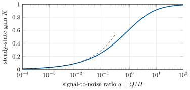
For the local level model with signal-to-noise ratio $q$, the predicted variance converges to $P = pH$ with $p = \frac12(q + \sqrt{q^2 + 4q})$, and the gain to $K = p/(1 + p)$. The filtered level is then an exponentially weighted average of past observations with weight $K$ on the newest.

For small $q$ the gain is about $\sqrt q$, so the filter’s memory is about $1/\sqrt q$ days and its half-life $\ln2/\sqrt q$ (Figure 19.1). The signal-to-noise ratio, not the analyst, decides how fast the filter reacts. For a regression coefficient the same holds with $q$ multiplied by the regressor’s mean square.

Definition 19.6 (Prediction-error decomposition)

The prediction-error decomposition writes the likelihood of the observations as the product of the one-step predictive densities, $\ln L = -\frac12\sum_t\bigl(\ln(2\pi F_t) + v_t^2/F_t\bigr)$, with the innovations and their variances from the filter.

The filter therefore delivers the likelihood of $(H, Q)$ at the cost of one pass, and maximum likelihood fits the noise variances. On the hedge, one more refinement matters: daily oil price changes are far from homoskedastic (the standard deviation of WTI’s was 0.78 dollars in 2017 and 3.62 in 2026), and a constant $H$ lets the volatile years dictate the fit. The chapter takes $\Var(\varepsilon_t) = H s_t^2$ with $s_t$ an exponentially weighted volatility of WTI’s changes known the day before, which is the same as filtering the scaled equation $\Delta b_t/s_t = \beta_t\Delta w_t/s_t + \varepsilon_t/s_t$.

19.3 A time-varying hedge ratio

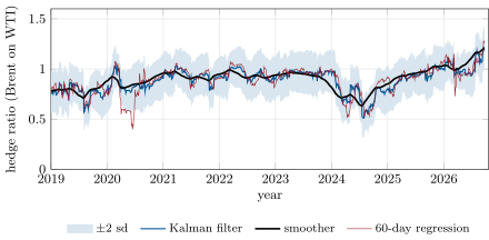
Fitted to the 4 097 daily changes from January 2010 to September 2026, the scaled model gives $H = 0.508$, $Q = 0.000238$ and a signal-to-noise ratio of 0.00047; with the scaled regressor’s mean square of 1.12, the filter’s half-response to a shift is $\ln2/\sqrt{0.00047 \times 1.12} = 30$ days, exactly the 30 days a 60-day window needs to cover half a shift. The filtered ratio’s uncertainty is itself large: its standard deviation is about 0.10, so the daily ratio is known only to $\pm 0.2$ (Figure 19.2).

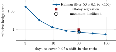
Each estimate hedges day $t$ with the ratio known at the close of day $t - 1$. Over the 4 035 days after a 60-day start, the mean squared hedge error, in dollars squared per barrel per day, is 3.324 unhedged, 1.329 with the ratio of the first 60 days held fixed, 1.276 with the 60-day regression and 1.267 with the Kalman filter: a reduction of 0.7% against the window. Without the volatility scaling, the maximum-likelihood filter is 1.4% worse than the window, because the volatile years push its $Q$ up tenfold. Making the filter faster is possible: multiplying $Q$ by 10 cuts the half-response to 9.6 days and raises the hedge error by 0.6% relative to the window; multiplying it by 100 gives 3.0 days and 6.2% more error (Figure 19.3). In a simulation where the ratio jumps from 0.7 to 1.0 with the fitted noise levels, the likelihood’s filter and the window both need about fifty days to reach 0.85; the filter with 100 times the $Q$ needs eight.

19.4 The smoother and expectation–maximisation

Definition 19.7 (Kalman smoother)

The Kalman smoother computes $\E[\alpha_t \mid y_1, \dots, y_n]$ and its variance from the filter’s output by a backward pass (Rauch, Tung and Striebel, 1965): $\hat\alpha_t = a_{t|t} + J_t(\hat\alpha_{t+1} - a_{t+1})$ with $J_t = P_{t|t}T^\top P_{t+1}^{-1}$.

The smoother answers a different question from the filter: not what the desk could have known, but what the ratio most likely was. It is the tool for research on past data (Figure 19.2 shows it smoother and earlier than the filter) and a source of look-ahead bias when it leaks into a backtest.

Definition 19.8 (Expectation–maximisation algorithm)

The expectation–maximisation algorithm (Dempster, Laird and Rubin, 1977) maximises a likelihood with unobserved variables by alternating an E-step, the expected complete-data log-likelihood given the data and the current parameters, and an M-step that maximises it. For state-space models the E-step is the smoother and the M-step for $H$ and $Q$ has a closed form (Shumway and Stoffer, 1982).

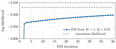
Each EM step cannot decrease the likelihood: the complete-data log-likelihood’s expectation is a lower bound on the log-likelihood, up to a constant, that touches it at the current parameters, and the M-step raises the bound. EM is stable and needs no derivatives, but it can be slow. Started from $H = 1$ and $Q = 0.01$ on the hedge model, it raises the log-likelihood from $-4\,947$ to $-4\,524$ in ten steps and to $-4\,502$ in forty, still 32 points short of the maximum $-4\,470$ that direct maximisation finds (Figure 19.4): the likelihood is flat along the direction that trades $Q$ against $H$.

19.5 Particle filters

Definition 19.9 (Particle filter, sequential importance resampling)

A particle filter represents the filtering law of a state by a weighted sample of particles. Sequential importance resampling, the bootstrap filter of Gordon, Salmond and Smith (1993), propagates each particle through the state equation, weights it by the density of the new observation given the particle, and resamples in proportion to the weights; the average weight at each step estimates the one-step predictive density, and their product the likelihood.

The particle filter needs neither linearity nor Gaussian noise, only the ability to simulate the state and evaluate the observation density; its price is Monte Carlo error and degeneracy, measured by the effective sample size of chapter 14 computed from the weights, $1/\sum_iw_i^2$. On a linear Gaussian local level of 500 observations, where the Kalman filter is exact, 2 000 particles give a log-likelihood of $-785.06$ against the exact $-784.22$ and filtered means within 0.07 of the exact ones (whose posterior standard deviation is 0.45), with an average effective sample size of 1 678.

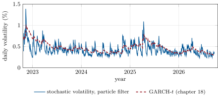
The useful case is nonlinear. A stochastic-volatility model for daily EUR/USD returns lets the log variance follow an AR(1), $x_t = \mu + \phi(x_{t-1} - \mu) + \sigma_\eta u_t$, and observes $r_t = e^{x_t/2}z_t$: no Kalman filter applies. With 5 000 particles on the last 1 000 returns, a grid search of the particle likelihood (same random numbers at every point) picks $\phi = 0.9$ and $\sigma_\eta = 0.4$ (log-likelihood $-568.4$, against $-572.3$ at $\phi = 0.95$, $\sigma_\eta = 0.2$: a flat surface). The filtered volatility follows the GARCH volatility of chapter 18 but reacts faster (Figure 19.5); the effective sample size averages 4 449 but falls to 23 on 3 April 2025, when the euro rose 2.7% after the US tariff announcement of 2 April (a risk-off episode in which, unusually, the dollar depreciated, as the ECB’s Financial Stability Review of November 2025 notes) and almost every particle was too calm to explain it.

19.6 Tutorial: the hedge ratio that moved

19.7 Build: the Kalman toolkit

19.8 Exercises

Exercise 19.1 ★

A local level model has $H = 1$ and $Q = 0.04$. What are the steady-state gain and the half-life of the filter’s memory?

Solution

Solution of Exercise 19.1.

$q = 0.04$: $p = (0.04 + \sqrt{0.0016 + 0.16})/2 = 0.221$ and $K = 0.221/1.221 = 0.181$. Old observations’ weights decay like $0.819^k$, which halves in $\ln\frac12/\ln0.819 = 3.5$ days.

Exercise 19.2 ★

Yesterday’s filtered hedge ratio is $0.80$ with variance $0.01$; $Q = 0.0002$, $H = 0.5$. Today WTI moves $+2$ and Brent $+1.2$ (scaled units). Update the ratio.

Solution

Solution of Exercise 19.2.

Predicted variance $0.01 + 0.0002 = 0.0102$. Innovation $v = 1.2 - 0.8 \times 2 = -0.4$, $F = 4 \times 0.0102 + 0.5 = 0.5408$, gain $K = 0.0102 \times 2/0.5408 = 0.0377$. Updated ratio $0.8 - 0.0377 \times 0.4 = 0.785$, variance $0.0102(1 - 0.0377 \times 2) = 0.0094$.

Exercise 19.3 ★

Why does a missing observation increase the state’s variance, and by how much in the local level model?

Solution

Solution of Exercise 19.3.

Without an observation there is no update, only the prediction step, which adds the state noise: in the local level model the variance grows by $Q$ that day, instead of first shrinking by the update. The uncertainty reflects that the state kept moving while nothing was seen.

Exercise 19.4 ★★

Show that for small $q$ the local level gain is approximately $\sqrt q$, and compare with an exponential moving average: which $\lambda$ does the filter imply for $q = 0.0004$?

Solution

Solution of Exercise 19.4.

For small $q$, $p = \frac12(q + \sqrt{q^2 + 4q}) \approx \sqrt q$ and $K = p/(1 + p) \approx \sqrt q$. The filtered level is $a_{t+1} = (1 - K)a_t + Ky_t$, an EMA with $\lambda = 1 - K$; for $q = 0.0004$, $K = 0.0198$ and $\lambda = 0.980$.

Exercise 19.5 ★★

Write the AR(1) plus noise, $y_t = x_t + \varepsilon_t$ with $x_t = \phi x_{t-1} + \eta_t$, in state-space form and give its steady-state predicted variance equation.

Solution

Solution of Exercise 19.5.

State $\alpha_t = x_t$, $Z = 1$, $T = \phi$, $Q = \Var(\eta)$, $H = \Var(\varepsilon)$. The steady predicted variance solves $P = \phi^2\bigl(P - P^2/(P + H)\bigr) + Q$.

Exercise 19.6 ★★

A particle filter’s normalised weights are 0.5, 0.3, 0.1, 0.05 and 0.05. What is the effective sample size?

Solution

Solution of Exercise 19.6.

$1/(0.25 + 0.09 + 0.01 + 0.0025 + 0.0025) = 1/0.355 = 2.8$ particles’ worth out of five.

Exercise 19.7 ★★★

Coding. On the Brent–WTI data, scale the fitted $Q$ by 0.1, 1, 10 and 100 and tabulate the hedge-error variance relative to the 60-day regression and the half-response time.

Solution

Solution of Exercise 19.7.

tradeoff(): $Q \times 0.1$: 0.987 of the window’s error, half-response 96 days; $\times 1$: 0.993, 30 days; $\times 10$: 1.006, 9.6 days; $\times 100$: 1.062, 3.0 days. Slower than the likelihood’s choice is marginally better here; faster costs noise.

Exercise 19.8 ★★★

Find the flaw. “We backtested a hedge using the Kalman-smoothed ratio and cut the hedge error by 15% against the rolling regression.”

Solution

Solution of Exercise 19.8.

The smoothed ratio for day $t$ uses prices after day $t$, so the backtest hedges with information the desk could not have had. Use the filtered ratio from the previous close; the smoother belongs to research on what the relationship was, not to a simulation of trading.

19.9 Problem: The Hedge Ratio That Moved

Problem 19.1

Weekend problem — how fast should a hedge ratio move?

The data are the EIA’s daily WTI and Brent spot prices from FRED, 4 January 2010 to 22 September 2026 (4 097 daily changes). Brent’s daily price change is hedged with WTI’s; the hedge ratio for day $t$ must be known at the close of day $t - 1$.

Part I — The data.

1. What happened on 20 April 2020, and how does the chapter treat it?
2. How did the yearly regression ratio move between 2014, 2021 and 2026?
3. Why scale the observation noise by WTI’s volatility?
4. What are the unhedged and the fixed-ratio hedge-error variances?
5. What does the 60-day regression achieve?

Part II — The filter.

6. What $H$, $Q$ and signal-to-noise ratio does maximum likelihood give?
7. What is the filter’s half-response to a shift, and how does it compare with the window’s?
8. What hedge-error variance does the filter achieve, and what reduction against the window?
9. What happens without the volatility scaling?
10. How precisely is the daily ratio known?

Part III — Speed and noise.

11. What do filters with $Q$ multiplied by 10 and by 100 achieve?
12. In the simulated jump from 0.7 to 1.0, how many days do the filters and the window need to reach 0.85?
13. What does EM find from a poor start, and why is it slow?
14. What are the filtered and rolling ratios at the end of the sample?
15. When would a fast filter be worth its noise?

Part IV — Judgement.

16. Should the desk replace its rolling regression?
17. What else could improve the hedge more than the choice of filter?
18. Why must the smoother stay out of the backtest?
19. State the named result: the reduction in hedge-error variance and the estimated signal-to-noise ratio.
20. In one sentence: what decides how fast a Kalman filter reacts?

Solution

Solution of Problem 19.1.

1. The EIA WTI spot price settled at $-36.98$ dollars; WTI changed by $-55.29$ and $+45.89$ on 20 and 21 April while Brent changed by $-2.39$ and $-8.24$. Both days are treated as missing: the filter skips the update, and the rolling regression and the evaluation skip the days. 2. 0.41 in 2014, 0.94 in 2021 and 1.01 in 2026. 3. WTI’s daily volatility ranged from 0.78 dollars (2017) to 3.62 (2026); with constant $H$ the volatile periods dominate the likelihood and push $Q$ up; scaling makes the observation noise closer to homoskedastic. 4. 3.324 unhedged and 1.329 with the first 60 days’ ratio held fixed (dollars squared per barrel per day, 4 035 days). 5. 1.276. 6. $H = 0.508$, $Q = 0.000238$, signal-to-noise ratio 0.00047. 7. $\ln2/\sqrt{0.00047 \times 1.12} = 30$ days, the same as the 60-day window’s 30. 8. 1.267, a reduction of 0.7%. 9. The fitted $Q$ is ten times larger (0.0026 against $H = 1.14$ in dollar units) and the filter hedges 1.4% worse than the window. 10. To about $\pm 0.2$: the filtered ratio’s standard deviation is about 0.10. 11. $\times 10$: 0.6% more error than the window, half-response 9.6 days; $\times 100$: 6.2% more, 3.0 days. 12. About fifty days for the likelihood’s filter (50) and for the window (49); eight days with 100 times the $Q$ (18 with ten times). 13. From $H = 1$, $Q = 0.01$ it reaches $-4\,524$ after ten steps and $-4\,502$ after forty, against the maximum $-4\,470$: the likelihood is flat along a ridge trading $Q$ against $H$, where EM’s steps are short. 14. Filtered 1.20, rolling 1.28 (22 September 2026). 15. When shifts are large and rare compared with the day’s noise (a structural break), which a random walk with Gaussian steps does not describe; a model with occasional jumps in the ratio, or a change-point detector, would react fast only when needed. 16. Only for the uncertainty band, the principled tuning and the handling of missing days; not for the hedge error, which is almost the same. 17. Synchronising the prices (the two spot assessments are taken at different times), adding WTI’s lagged change, and hedging with futures rather than spot prices. 18. Because it uses future data: any backtest with it hedges with hindsight. 19. Named result: the hedge ratio that moved: on 2010–2026 data the maximum-likelihood Kalman hedge ratio reduces the hedge-error variance by 0.7% against the 60-day rolling regression, with an estimated signal-to-noise ratio of 0.00047, which makes the filter as slow as the window. 20. The ratio of the state’s noise to the observation noise, which the likelihood estimates from the data.

19.10 Interview questions

Interview question 19.1 ★ researcher, trader

Explain the Kalman filter to a trader in three sentences.

Solution

Solution of Interview question 19.1.

You believe something you cannot see, like a hedge ratio, drifts slowly; each day you predict it, see how wrong the prediction of today’s prices was, and move your belief toward the evidence by a fraction that depends on how noisy the prices are compared with how fast the hidden thing moves. You also track how uncertain your belief is. It is the optimal way to do this when everything is linear and Gaussian.

What the interviewer is looking for: Predict, compare, correct in proportion to relative noise, and carry the uncertainty.

Interview question 19.2 ★★ researcher

Derive the Kalman update for a scalar state from Gaussian conditioning.

Solution

Solution of Interview question 19.2.

Prior $\alpha \sim \mathcal N(a, P)$, observation $y = z\alpha + \varepsilon$, $\varepsilon \sim \mathcal N(0, H)$. $(\alpha, y)$ are jointly normal with $\Cov = Pz$ and $\Var(y) = z^2P + H$. Conditioning: $a' = a + \frac{Pz}{z^2P + H}(y - za)$ and $P' = P - \frac{P^2z^2}{z^2P + H}$; the gain is $K = Pz/(z^2P + H)$.

What the interviewer is looking for: The joint-normal argument, not a memorised formula.

Interview question 19.3 ★★ researcher, trader

How do you choose the process noise of a Kalman filter tracking a hedge ratio?

Solution

Solution of Interview question 19.3.

Estimate it with the observation noise by maximum likelihood from the prediction-error decomposition, then check the hedge out of sample and the speed-noise trade-off; choosing it by hand to “react in days” buys noise. Scale the observation noise with volatility first, or the fit is dominated by volatile periods.

What the interviewer is looking for: Likelihood-based tuning, the trade-off, and heteroskedasticity.

Interview question 19.4 ★★ researcher, mle

What is the difference between filtering and smoothing, and why does it matter in backtests?

Solution

Solution of Interview question 19.4.

Filtering conditions on data up to $t$; smoothing on all data, past and future. The smoothed path is better for describing history and wrong for trading simulations, where it is look-ahead bias.

What the interviewer is looking for: Information sets and look-ahead bias.

Interview question 19.5 ★★ mle, researcher

When would you use a particle filter instead of a Kalman filter, and what can go wrong?

Solution

Solution of Interview question 19.5.

When the model is nonlinear or non-Gaussian: stochastic volatility, jumps, heavy-tailed noise, discrete regimes. It can degenerate (few particles carry the weight) on surprising observations, its likelihood is noisy (which complicates parameter estimation), and its cost grows with the state dimension.

What the interviewer is looking for: Nonlinearity as the reason, degeneracy and Monte Carlo noise as the risks, effective sample size as the monitor.

Interview question 19.6 ★★★ researcher

Why does each EM iteration not decrease the likelihood?

Solution

Solution of Interview question 19.6.

For any law $q$ of the hidden variables, $\ln p(y \mid \theta) = \E_q[\ln p(y, \alpha \mid \theta)] - \E_q[\ln q] + \mathrm{KL}(q\,\|\,p(\alpha \mid y, \theta))$. The E-step sets $q$ to the posterior at $\theta_k$, making the KL term zero, so the bound touches the likelihood there; the M-step raises the bound; the likelihood at $\theta_{k+1}$ is at least the raised bound, hence at least the likelihood at $\theta_k$.

What the interviewer is looking for: The lower bound and the KL gap.