2Brownian Motion

A trader buys a stock with an annual volatility of 30% and places a stop-loss 2% below the entry price, then asks the risk desk how likely the stop is to be touched within a month. The chance that the stock merely ends the month below the stop is 41%; the chance that it touches the stop at some moment of the month is exactly twice that, 82%. If the stop is checked only at each day’s close, the answer is 72%, and a simulation that watches the closes and forgets what happens between them reports 72% for a contract that is really triggered 82% of the time. The three numbers come from one object, the Brownian motion, and from three of its properties: its law at a fixed time, the reflection principle for its running minimum, and the Brownian bridge that describes it between two observations. This chapter builds the object, proves the properties the series uses, and ends with the quadratic variation, the property that makes stochastic calculus different from the ordinary kind.

2.1 From random walks to Brownian motion

Definition 2.1 (Brownian motion, Gaussian process)

A Gaussian process is a process $(X_t)$ whose finite-dimensional laws $(X_{t_1}, \dots, X_{t_k})$ are all multivariate normal; its law is fixed by its mean $m(t)$ and covariance $c(s,t)$. A (standard) Brownian motion $(W_t)_{t \ge 0}$ is an adapted process with $W_0 = 0$, continuous paths, and increments $W_t - W_s$ independent of $\mathcal F_s$ and distributed $\mathcal N(0, t - s)$ for $s < t$.

Equivalently, $W$ is the centred Gaussian process with continuous paths and covariance $c(s,t) = \min(s,t)$: for $s < t$, $\Cov(W_s, W_t) = \Cov(W_s, W_s + (W_t - W_s)) = s$. Existence is not obvious, since the definition asks for continuity of uncountably many random variables at once. Wiener gave the first construction in 1923; the one that serves simulation builds the path coarse to fine (Section 2.5). The reason Brownian motion appears everywhere is a central limit theorem for paths.

Theorem 2.2 (Donsker’s invariance principle)

Let $\xi_1, \xi_2, \dots$ be independent and identically distributed with mean zero and variance one, $S_k = \sum_{i \le k}\xi_i$, and $X^{(n)}_t = n^{-1/2}(S_{\lfloor nt\rfloor} + (nt - \lfloor nt\rfloor)\xi_{\lfloor nt\rfloor + 1})$ the linearly interpolated, rescaled walk. Then $X^{(n)} \xrightarrow{d} W$ as random elements of $C[0, 1]$: $\E[F(X^{(n)})] \to \E[F(W)]$ for every bounded continuous functional $F$ of the path.

Donsker’s theorem is what licenses the use of Brownian motion for prices built from many small, independent trades, whatever their individual law: the maximum of the path, the time spent below a level, the average price, all continuous functionals, converge together. It does not license it for prices driven by a few large jumps (chapter 6).

Proposition 2.3 (Invariances)

If $W$ is a Brownian motion, so are $-W_t$; $c^{-1/2}W_{ct}$ for every $c > 0$ (scaling); $W_{s+t} - W_s$ for fixed $s$; and $tW_{1/t}$ (with value 0 at $t = 0$).

Scaling is the square-root-of-time rule a trader uses without thinking: a stock with 30% annual volatility has a one-day standard deviation of $0.30/\sqrt{252} = 1.9\%$ and a one-month one of $0.30\sqrt{21/252} = 8.7\%$. Figure 2.1 shows six paths inside the envelope $\pm 2\sqrt t$.

2.2 Path properties and the Markov property

Brownian paths are continuous and nowhere smooth. Almost surely they are Hölder continuous of every order $\alpha < \tfrac12$ and of no order $\alpha > \tfrac12$, and differentiable at no point; they cross any level they touch infinitely often immediately afterwards. None of this is pathology for its own sake: it is the reason a hedge rebalanced continuously in time still accumulates a nonzero cost (chapter 3), and the reason a barrier touched once is touched many times.

Definition 2.4 (Markov process, strong Markov property)

An adapted process $(X_t)$ is a Markov process if for all $s, t \ge 0$ and bounded measurable $f$, $\E[f(X_{s+t}) \mid \mathcal F_s] = \E[f(X_{s+t}) \mid X_s]$: given the present, the past adds nothing. It has the strong Markov property if the same holds with $s$ replaced by any finite stopping time $\tau$.

Theorem 2.5 (Brownian motion is strong Markov)

For every stopping time $\tau$ with $\P(\tau < \infty) = 1$, the process $B_t = W_{\tau + t} - W_\tau$ is a Brownian motion independent of $\mathcal F_\tau$.

The proof approximates $\tau$ from above by stopping times with countably many values, for which the statement is the simple Markov property applied on each value (Karatzas and Shreve, 1991, §2.6). The strong Markov property is what makes the next section work: after the first time a path reaches a level, what it does next is a fresh Brownian motion, as likely to go up as down.

2.3 The reflection principle and first-passage times

Definition 2.6 (First-passage time)

For a level $b$, the first-passage time (or hitting time) of a continuous process $X$ is $\tau_b = \inf\{t \ge 0 : X_t = b\}$; it is a stopping time.

Theorem 2.7 (Reflection principle)

For $b > 0$ and $t > 0$, let $M_t = \max_{s \le t}W_s$. Then

$$\P(M_t \ge b) = \P(\tau_b \le t) = 2\P(W_t \ge b) = 2\bigl(1 - \Phi(b/\sqrt t)\bigr),$$

and more precisely $\P(M_t \ge b, W_t \le a) = \P(W_t \ge 2b - a)$ for $a \le b$.

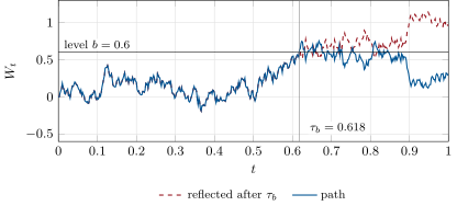
Differentiating in $t$ gives the law of the first-passage time: $\tau_b$ has density $b(2\pi t^3)^{-1/2}e^{-b^2/2t}$, finite almost surely but with infinite mean, since the density decays like $t^{-3/2}$. A driftless price reaches any level eventually, and one should not wait for it. The stop of the hook is the reflection principle applied to the log price.

Definition 2.8 (Brownian motion with drift)

A Brownian motion with drift $\mu$ and volatility $\sigma > 0$ is $X_t = \mu t + \sigma W_t$.

Proposition 2.9 (First passage with drift)

For $X_t = \mu t + \sigma W_t$ and $b < 0$,

$$\P\bigl(\min_{s \le T}X_s \le b\bigr) = \Phi\Bigl(\frac{b - \mu T}{\sigma\sqrt T}\Bigr) + e^{2\mu b/\sigma^2}\,\Phi\Bigl(\frac{b + \mu T}{\sigma\sqrt T}\Bigr).$$

The proof changes the measure to remove the drift and applies the reflection principle (an exercise of chapter 5 derives it). For the hook, $b = \ln 0.98 = -0.0202$ and $\sigma\sqrt T = 0.0866$: without drift the stop is touched with probability $2\Phi(-0.233) = 81.6\%$; with the drift $-\sigma^2/2$ that makes the price itself a martingale, 82.4%.

Proposition 2.10 (Discrete monitoring: the Broadie–Glasserman–Kou shift)

If $X$ is observed only at times $k\Delta t$, the probability that an observation falls at or below $b < 0$ is, to first order in $\sqrt{\Delta t}$, the continuous probability for the shifted level $b - \beta\sigma\sqrt{\Delta t}$, with $\beta = -\zeta(\tfrac12)/\sqrt{2\pi} \approx 0.5826$.

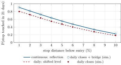
The shift is the mean overshoot of the path beyond the level at the first observation below it (Broadie, Glasserman and Kou, 1997). With daily closes, $\beta\sigma\sqrt{\Delta t} = 0.0110$: the 2% stop behaves like a 3.1% stop watched continuously, and is touched with probability 71.9%, against 72.0% in a simulation of 200 000 months of daily closes. Figure 2.3 shows the three curves over stop distances from 1% to 10%. The error of discrete monitoring shrinks only like $\sqrt{\Delta t}$: refining a daily simulation to four, sixteen and sixty-four observations a day gives 77.1%, 79.1% and 80.5% against the continuous 81.6%, the gap roughly halving each time the step is divided by four. A simulation that wants the continuous answer should not refine the grid; it should use the bridge of Section 2.5.

2.4 Quadratic variation

Definition 2.11 (Quadratic variation)

The quadratic variation of a process $X$ on $[0, t]$ is the limit in probability $[X]_t = \lim\sum_k (X_{t_{k+1}} - X_{t_k})^2$ over partitions $0 = t_0 < \dots < t_n = t$ whose mesh $\max_k(t_{k+1} - t_k)$ tends to zero, when it exists.

Theorem 2.12 (Quadratic variation of Brownian motion)

$[W]_t = t$: the sums converge to $t$ in $L^2$, and almost surely along dyadic partitions. Consequently the total variation $\sum_k|W_{t_{k+1}} - W_{t_k}|$ tends to infinity.

For a smooth function the sum of squared increments vanishes; for a Brownian path it is the elapsed time, deterministically, whichever path occurs. For $\sigma W$ it is $\sigma^2 t$, so one path observed ever more finely reveals its volatility exactly, while its drift stays unobservable over any fixed period: the reason realised volatility (One Quant Book 1, chapter 25) is estimated so much better than an expected return, and the reason the microstructure noise of chapter 21 matters so much. Figure 2.4 samples one path at $4$ to $65\,536$ points.

2.5 The Brownian bridge

Definition 2.13 (Brownian bridge)

A Brownian bridge from $x$ to $y$ on $[t_0, t_1]$ is a Brownian motion conditioned on $W_{t_0} = x$ and $W_{t_1} = y$; from $0$ to $0$ on $[0, T]$ it can be written $W_t - (t/T)W_T$, a centred Gaussian process with covariance $s(T - t)/T$ for $s \le t$.

Proposition 2.14 (What happens between two observations)

Given $W_{t_0} = x$ and $W_{t_1} = y$, with $h = t_1 - t_0$: (i) $W_s$ for $t_0 < s < t_1$ is normal with mean $x + (s - t_0)(y - x)/h$ and variance $(s - t_0)(t_1 - s)/h$, in particular $\mathcal N((x+y)/2, h/4)$ at the midpoint; (ii) for $\sigma W$ and a level $b$ below both $x$ and $y$,

$$\P\bigl(\min_{t_0 \le s \le t_1}\sigma W_s \le b \bigm| \sigma W_{t_0} = x, \sigma W_{t_1} = y\bigr) = \exp\Bigl(-\frac{2(x - b)(y - b)}{\sigma^2 h}\Bigr).$$

Method 2.15 (Two uses of the bridge in simulation)

(i) Building paths coarse to fine: draw $W_T = \sqrt T Z_0$, then the midpoint of each interval from part (i), halving the intervals until the grid is fine enough. The path has the right law, and the first normals fix its large-scale shape, which chapter 26 exploits with low-discrepancy points. (ii) Monitoring a barrier between grid points: simulate the path at the observation dates only, and for each interval multiply the probabilities $1 - p_k$ of not crossing, with $p_k$ from part (ii). One minus the product is an unbiased estimate of the continuous crossing probability, with no grid refinement.

Two closes each 1% above the stop, one day apart at 30% volatility, leave a 57% chance that the stop was touched in between: $\exp(-2 \times 0.01^2/(0.09/252))$. The simulation of Figure 2.3 that adds these probabilities to daily closes recovers the continuous answer, 81.6%, with no finer grid.

2.6 Tutorial: stops, reflections and quadratic variation

2.7 Build: the Monte Carlo engine, stage one

2.8 Exercises

Exercise 2.1 ★

Compute $\Cov(W_2, W_5)$, $\Var(W_5 - W_2)$ and the correlation of $W_2$ and $W_5$.

Solution

Solution of Exercise 2.1.

$\Cov(W_2, W_5) = \min(2,5) = 2$; $\Var(W_5 - W_2) = 3$; correlation $2/\sqrt{2 \times 5} = 0.632$.

Exercise 2.2 ★

What is the probability that a standard Brownian motion reaches 1 before time 1?

Solution

Solution of Exercise 2.2.

By the reflection principle, $\P(M_1 \ge 1) = 2(1 - \Phi(1)) = 31.7\%$.

Exercise 2.3 ★

A stock has an annual volatility of 20%. What is the standard deviation of its log return over one day and over one week of five trading days?

Solution

Solution of Exercise 2.3.

$0.20/\sqrt{252} = 1.26\%$ a day; $\sqrt5$ times that, 2.82%, a week.

Exercise 2.4 ★★

A stop sits 5% below the entry of a stock with 30% volatility. What is the probability it is touched within three months (63 trading days) if watched continuously, and if watched at the closes only?

Solution

Solution of Exercise 2.4.

$b = \ln 0.95 = -0.0513$, $T = 0.25$: continuously $2\Phi(b/0.15) = 73.2\%$; at the closes, the level shifted by $0.0110$ gives 67.8%.

Exercise 2.5 ★★

Show that $W_t^2 - t$ is a martingale, and deduce the expected time for $W$ to leave the interval $(-a, b)$, $a, b > 0$.

Solution

Solution of Exercise 2.5.

$\E_s[W_t^2] = W_s^2 + (t - s)$, so $W_t^2 - t$ is a martingale. With $\tau$ the exit time, $\E[W_{\tau\wedge n}^2] = \E[\tau \wedge n]$; letting $n \to \infty$ (bounded convergence on the left, monotone on the right) and using $\P(W_\tau = b) = a/(a+b)$: $\E[\tau] = b^2\frac{a}{a+b} + a^2\frac{b}{a+b} = ab$.

Exercise 2.6 ★★

For a Brownian bridge from 0 to 0 on $[0, 1]$, give the law of its value at $t = \tfrac12$ and the probability that it reaches $0.5$.

Solution

Solution of Exercise 2.6.

$\mathcal N(0, \tfrac14)$, from the covariance $s(1 - s)$; by Proposition 2.14, $\P(\max \ge 0.5) = \exp(-2 \times 0.5 \times 0.5) = 60.7\%$.

Exercise 2.7 ★★★

Coding. The sum of squared increments of $W$ on $[0,1]$ at $n$ points has standard deviation $\sqrt{2/n}$. Check it by simulating 2 000 paths at $n = 4\,096$, and say whether the fluctuations of Figure 2.4 are consistent with it.

Solution

Solution of Exercise 2.7.

$\Var(\sum\Delta_k^2) = \sum 2(1/n)^2 = 2/n$: at $n = 4\,096$ the standard deviation is 0.022, and 2 000 simulated paths give 0.022. The figure’s value at 4 096 points, 1.031, is 1.4 standard deviations from 1: consistent.

Exercise 2.8 ★★★

Find the flaw. “Our Monte Carlo for a contract that knocks out if the stock ever trades below a barrier simulates daily closes and checks them against the barrier; the price has converged to four digits.” Correct it.

Solution

Solution of Exercise 2.8.

Checking daily closes prices a contract monitored daily, not continuously: it misses every crossing between closes and underestimates the knock-out probability by several points (72% against 82% for the 2% stop of the chapter). More paths only reduce the statistical error, not this bias, which falls like $\sqrt{\Delta t}$. Add each interval’s bridge crossing probability, or price the continuous contract with the level shifted by $\beta\sigma\sqrt{\Delta t}$ to check.

2.9 Problem: The Stop-Loss

Problem 2.1

Weekend problem — how often a 2% stop is touched in a month

A stock with an annual volatility of 30% is bought with a stop 2% below the entry. Its log price is modelled as a Brownian motion with volatility $\sigma = 0.30$ and no drift, over 21 trading days of a 252-day year.

Part I — The continuous stop.

1. What is the stop level $b$ in log price, and the standard deviation $\sigma\sqrt T$ over the month?
2. What is the probability that the stock ends the month below the stop?
3. What is the probability that it touches the stop during the month, watched continuously?
4. Why is the second number exactly twice the first?
5. With the drift $-\sigma^2/2$ that makes the price a martingale, what does Proposition 2.9 give?

Part II — Watched at the close.

6. What does a simulation of 200 000 months of daily closes give?
7. What is the Broadie–Glasserman–Kou shift with daily closes, and the equivalent continuous stop?
8. What probability does the shifted level give?
9. Watched every 15 minutes (26 times a day), what do the simulation and the shift give?
10. Why does refining the grid by four only halve the gap to the continuous answer?

Part III — The bridge.

11. Two consecutive closes are each 1% above the stop. What is the probability the stop was touched between them?
12. What does the daily simulation give once each day’s crossing probability is added?
13. Why is this estimate unbiased for the continuous probability?
14. Which is cheaper for a target accuracy: 64 observations a day, or daily observations with the bridge?

Part IV — Judgement.

15. At 15% volatility, what is the continuous probability?
16. Over three months, what are the continuous and daily-close probabilities?
17. The stop is a resting order on the exchange; which number applies, and what does the model miss?
18. The desk sells a note that knocks out on a daily close below the level. Which number should price it?
19. State the named result: the probability that the 2% stop is touched in a month, continuously and at the closes.
20. In one sentence: why is a barrier watched continuously so much more likely to be touched than one watched daily?

Solution

Solution of Problem 2.1.

1. $b = \ln 0.98 = -0.0202$; $\sigma\sqrt T = 0.30\sqrt{21/252} = 0.0866$. 2. $\Phi(-0.0202/0.0866) = \Phi(-0.233) = 40.8\%$. 3. $2 \times 40.8\% = 81.6\%$. 4. By the reflection principle each path that touches the stop and ends above it is paired with its mirror image, which ends below. 5. 82.4%: the negative drift makes the touch slightly likelier. 6. 72.0% (standard error 0.1 point). 7. $0.5826 \times 0.30/\sqrt{252} = 0.0110$ in log price: the stop behaves like a 3.1% stop watched continuously. 8. 71.9%. 9. 79.6% by simulation, 79.6% by the shift. 10. The overshoot, and hence the error, is of order $\sigma\sqrt{\Delta t}$: dividing $\Delta t$ by four halves it (77.1%, 79.1%, 80.5% at 4, 16 and 64 observations a day). 11. $\exp(-2 \times 0.01 \times 0.01/(0.09/252)) = 57.1\%$. 12. 81.6% (standard error 0.08 point), equal to the continuous answer. 13. Given the closes, the crossings in different days are independent bridges, so $1 - \prod(1 - p_k)$ is the conditional probability of a touch; its mean is the unconditional one. 14. The bridge: it is exact at the cost of daily steps, while 64 steps a day still leave a 1-point bias at 64 times the cost. 15. 64.1%. 16. 89.3% continuously, 83.5% at the closes. 17. The continuous number, 82%; the model misses gaps (the order fills below the stop when the price jumps through it), volatility that is not constant, and intraday patterns. 18. The daily-close number, 72%: the contract is monitored at the closes. 19. Named result: the stop-loss: a 2% stop on a 30%-volatility stock is touched within a month with probability 81.6% if watched continuously and 72.0% if watched at the closes; the Broadie–Glasserman–Kou shift gives 71.9% and the bridge-corrected daily simulation 81.6%. 20. Because a Brownian path crosses and re-crosses a level between observations, and the closes see only the crossings that last until the close.

2.10 Interview questions

Interview question 2.1 ★ trader, researcher

A driftless Brownian motion starts at 0. What is the probability it hits $-1$ before $+2$?

Solution

Solution of Interview question 2.1.

$W$ is a bounded martingale up to the exit, so $\E[W_\tau] = 0$: $-1 \times p + 2(1 - p) = 0$, $p = 2/3$.

What the interviewer is looking for: optional stopping in one line.

Interview question 2.2 ★ researcher

Why is the quadratic variation of a Brownian path $t$, and why does it matter for trading?

Solution

Solution of Interview question 2.2.

The squared increments over a partition have mean equal to the elapsed time and a variance that vanishes with the mesh. It is why the variance of a hedged book accumulates with time whatever the rebalancing frequency, why volatility is measurable from one path, and why Itô’s formula has a second-order term.

What the interviewer is looking for: the $L^2$ computation and its consequences.

Interview question 2.3 ★★ researcher, trader

What is the expected maximum of a standard Brownian motion over $[0,1]$?

Solution

Solution of Interview question 2.3.

By the reflection principle $M_1$ has the law of $|W_1|$, so $\E[M_1] = \sqrt{2/\pi} = 0.798$.

What the interviewer is looking for: reflection, then the half-normal mean.

Interview question 2.4 ★★ developer, researcher

How do you price a continuously monitored barrier by Monte Carlo without taking tiny time steps?

Solution

Solution of Interview question 2.4.

Simulate on the grid you need anyway and, in each interval, multiply by the bridge probability of not crossing, $1 - \exp(-2(x_k - b)(x_{k+1} - b)/\sigma^2\Delta t)$ (or sample the crossing with that probability); for a quick check, shift the level by $0.5826\,\sigma\sqrt{\Delta t}$.

What the interviewer is looking for: the Brownian-bridge crossing probability.

Interview question 2.5 ★★ risk, trader

A trader says a 2% stop on a 30%-volatility stock is triggered about 40% of the time in a month. What did they compute, and what is the right number?

Solution

Solution of Interview question 2.5.

The probability of ending the month below the stop, 41%. A stop is triggered by the minimum, not the terminal value; by reflection the right number is twice that, 82% continuously, 72% if only closes count.

What the interviewer is looking for: terminal versus path-dependent probability.

Interview question 2.6 ★★★ researcher

Compute $\P(W_1 > 0, W_2 > 0)$.

Solution

Solution of Interview question 2.6.

$(W_1, W_2 - W_1)$ are independent standard normals $(X, Y)$, and the event is $X > 0$, $X + Y > 0$: a wedge of angle $\pi/2 + \pi/4$ in the plane, so the probability is $(3\pi/4)/(2\pi) = 3/8$.

What the interviewer is looking for: rotational symmetry of the Gaussian.