28Transforms, Interpolation and Algorithmic Differentiation

The risk run bumps 400 curve points one at a time and reprices the book 401 times every night. The same 400 sensitivities come out of one recording of the pricing code and one sweep backwards through it, at the cost of a few prices. This chapter collects the numerical tools that pricing and risk code is made of: Fourier methods that price from a characteristic function, interpolation that turns a handful of quotes into a curve, root finders that invert a pricing formula, and algorithmic differentiation, which delivers exact derivatives of whatever the code computes.

28.1 Fourier methods

Definition 28.1 (Discrete and fast Fourier transforms)

The discrete Fourier transform of $x_0, \dots, x_{N-1}$ is $X_k = \sum_{j=0}^{N-1}x_je^{-2\pi\mathrm ijk/N}$, $k = 0, \dots, N - 1$. A fast Fourier transform computes it in $O(N\log N)$ operations instead of $O(N^2)$ by splitting it recursively into transforms of half the length (Cooley and Tukey, 1965).

A Lévy model is specified by its characteristic exponent (chapter 6), not its density, so prices come from the characteristic function $\varphi(u) = \E[e^{\mathrm iu\ln(S_T/S_0)}]$. Carr and Madan (1999) price a whole strip of strikes with one fast Fourier transform of a damped call; the method below needs no damping and converges faster.

Proposition 28.2 (Fourier inversion)

For a random variable $X$ with characteristic function $\varphi$ and a continuity point $k$ of its distribution, $\P(X > k) = \frac12 + \frac1\pi\int_0^\infty\mathrm{Re}\bigl[e^{-\mathrm iuk}\varphi(u)/(\mathrm iu)\bigr]\,du$ (Gil-Pelaez, 1951).

For a Merton jump diffusion ($\sigma = 15\%$, jumps at rate 0.5 a year with mean $-0.1$ and standard deviation 0.2 in log-price, $r = 3\%$, one year), the formula with the trapezoidal rule on $[0, 200]$ gives $\P(S_T > 110) = 0.3503999$, against the Poisson mixture of lognormals to $3 \times 10^{-10}$.

Definition 28.3 (COS method)

The COS method (Fang and Oosterlee, 2008) truncates the density of $y = \ln(S_T/K)$ to an interval $[a, b]$, expands it in a cosine series whose coefficients are read off the characteristic function, $A_k \approx \frac2{b-a}\mathrm{Re}[\varphi(\frac{k\pi}{b-a})e^{-\mathrm ik\pi a/(b-a)}]$, and integrates the payoff against each cosine in closed form, so that a price is $e^{-rT}\sum_{k<N}{}'A_kV_k$ (the first term halved).

Proposition 28.4 (Convergence of the COS method)

For a density that is smooth on the truncation interval, the cosine coefficients decay faster than any power of $k$, and the error of the COS price decays exponentially in $N$ until the truncation error of $[a, b]$ dominates (Fang and Oosterlee, 2008; stated).

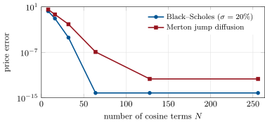
With $[a, b]$ set by ten standard deviations from the cumulants, a Black–Scholes call is exact to $7 \times 10^{-15}$ with 64 terms, and the Merton call to $10^{-7}$ with 64 and $2 \times 10^{-12}$ with 128 (Figure 28.1). The firm prices calls from the put expansion and parity, which keeps the coefficients bounded. For a variance-gamma model, where only simulation is available as a check, 256 terms give 9.5243 and 400 000 simulated paths $9.528 \pm 0.022$.

28.2 Interpolation and splines

Definition 28.5 (Cubic, natural and monotone splines, Runge phenomenon)

A cubic spline through $(x_i, y_i)$ is a piecewise cubic with continuous first and second derivatives; a natural cubic spline has zero second derivative at both ends, and its second derivatives at the nodes solve a tridiagonal system. Monotone cubic interpolation chooses the node slopes of a piecewise cubic Hermite interpolant so that it is monotone wherever the data are. The Runge phenomenon (Runge, 1901) is the growth, near the ends of the interval, of the error of polynomial interpolation at equally spaced nodes as the degree increases.

Proposition 28.6 (Minimal curvature of the natural spline)

Among all twice continuously differentiable functions through the data, the natural cubic spline minimises $\int(f^{\prime\prime})^2$.

Proposition 28.7 (Fritsch–Carlson condition)

On an interval where the data increase with secant slope $\delta > 0$, the cubic Hermite interpolant with end slopes $m_0, m_1 \ge 0$ is monotone if $\alpha = m_0/\delta$ and $\beta = m_1/\delta$ satisfy $\alpha^2 + \beta^2 \le 9$ (Fritsch and Carlson, 1980).

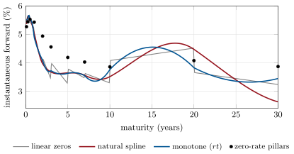
Minimal curvature is not what a rates desk wants. On the Treasury curve of 3 July 2023 (constant-maturity yields from one month to thirty years, treated as zero rates for the illustration), the natural spline of the zero rates produces a forward curve that falls to 2.63% at thirty years; the monotone interpolation of $rt$, whose derivative is the forward, keeps every forward between 3.32% and 5.67%; linear interpolation of zero rates gives forwards that jump by up to 0.43 percentage points at the pillars (Figure 28.2). Hagan and West (2006) survey the methods used for curves. Global polynomials are worse still: through eleven equally spaced samples of $1/(1 + 25x^2)$ on $[-1, 1]$, the interpolating polynomial errs by 1.92 near the ends.

28.3 Root finding

Definition 28.8 (Bisection, secant and Brent’s methods)

The bisection method halves a bracket $[a, b]$ with $f(a)f(b) < 0$ at each step. The secant method replaces the derivative in Newton’s method by the slope through the last two iterates. Brent’s method (Brent, 1973) keeps a bracket and takes an inverse quadratic interpolation or secant step when it stays inside the bracket and shrinks it fast enough, and a bisection step otherwise.

Proposition 28.9 (Convergence of the root finders)

Bisection gains one bit per step and always converges; the secant method converges locally with order $(1 + \sqrt5)/2 \approx 1.618$ at a simple root; Brent’s method always converges, never much more slowly than bisection (at most about the square of the bisection count), and superlinearly near a simple root (Brent, 1973).

Implied volatility is the standard test. For a one-year call ($S = 100$, $r = 3\%$, true volatility 25%), bisection on $[0.001, 5]$ needs 36 steps at every strike. At the money, Newton from 20% needs 3 iterations, the secant method 4, Brent 5. At a strike of 400 the price is $2.5 \times 10^{-7}$ and the vega at 20% is $8 \times 10^{-9}$: Newton’s first step goes to a volatility of 3 062%, where the vega underflows, and the secant method also fails, while Brent converges in 18. The firm’s rule is a bracketing method with a fast interior step, and Newton only from a guess known to be close.

28.4 Forward and adjoint algorithmic differentiation

Definition 28.10 (Algorithmic differentiation, forward and reverse modes, dual numbers)

Algorithmic differentiation computes derivatives of a function given as a program by applying the chain rule to its elementary operations, exactly up to rounding. Forward mode propagates, with each value, its derivative along one input direction; dual numbers $a + b\epsilon$ with $\epsilon^2 = 0$ implement it, since $f(a + b\epsilon) = f(a) + f'(a)b\epsilon$ (Wengert, 1964). Reverse mode records the operations and then propagates adjoints $\bar v = \partial y/\partial v$ from the output back to every input (Linnainmaa, 1976, from his 1970 master’s thesis on rounding errors; Griewank, 2012, recounts several independent discoveries); in finance it is called adjoint mode, or AAD.

Definition 28.11 (Tape, checkpointing)

A tape is the record, made during the forward evaluation, of each elementary operation’s inputs and local partial derivatives. Checkpointing stores only some intermediate states during the forward pass and recomputes the operations between them during the reverse pass, trading computation for memory.

Proposition 28.12 (Cheap gradient principle)

For a scalar function of $n$ inputs evaluated with $E$ elementary operations, each with at most two inputs, the reverse mode computes the whole gradient with a number of operations bounded by a small constant times $E$, independent of $n$; forward mode and finite differences need $n$ passes (Griewank and Walther, 2008).

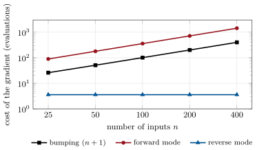
The firm’s toy book has 400 zero-rate pillars on thirty years, 120 quarterly cash flows and 119 caplets priced by Black’s formula on the three-month forwards: 2 864 operations for one value. The reverse sweep costs, in the count above, 3.58 evaluations; bumping costs 401 and forward mode 1 433 (Figure 28.3). The adjoint gradient agrees with forward mode to $2 \times 10^{-13}$ and with central differences to $9 \times 10^{-6}$ on sensitivities as large as 517 (the bumps’ own error); 213 of the 400 are nonzero, since only the pillars next to a cash-flow date matter under linear interpolation. The C++20 twin, timed in its acceptance test, returns the gradient of a similar 400-input function in less than twenty times one plain evaluation (between five and seven in the runs made for this chapter, tape allocation included).

The price of the reverse mode is memory: the tape holds every operation. A time-stepping loop of 10 000 steps records 60 003 nodes; with a checkpoint every 100 steps, the reverse pass holds at most 201 states (100 checkpoints and one segment) and recomputes the loop once, and the gradient is the same to $10^{-14}$. Two practical cautions: a payoff with a kink or a jump has a derivative that is zero or undefined almost everywhere, so AAD of a Monte Carlo digital returns zero and needs smoothing or a likelihood-ratio term; and code that branches on values records only the branch taken. Giles and Glasserman (2006) brought the adjoint method to Monte Carlo Greeks in finance.

28.5 Tutorial: one sweep instead of 401

28.6 Build: algorithmic differentiation

28.7 Exercises

Exercise 28.1 ★

How many complex multiplications does a direct discrete Fourier transform of length 4 096 need, and roughly how many does a radix-2 fast Fourier transform need?

Solution

Solution of Exercise 28.1.

Directly $N^2 = 16\,777\,216$; radix 2 about $\frac N2\log_2N = 2\,048 \times 12 = 24\,576$, some 700 times fewer.

Exercise 28.2 ★

Evaluate $f(x) = x^2e^x$ on the dual number $1 + \epsilon$ and read off $f'(1)$.

Solution

Solution of Exercise 28.2.

$(1 + \epsilon)^2 = 1 + 2\epsilon$ and $e^{1+\epsilon} = e + e\epsilon$, so $f(1 + \epsilon) = (1 + 2\epsilon)(e + e\epsilon) = e + 3e\epsilon$: $f'(1) = 3e \approx 8.155$.

Exercise 28.3 ★

How many bisection steps reduce a bracket of width 5 below $10^{-10}$?

Solution

Solution of Exercise 28.3.

$5 \cdot 2^{-k} < 10^{-10}$ needs $k > \log_2(5 \times 10^{10}) = 35.5$: 36 steps, as in the tutorial.

Exercise 28.4 ★★

Write the tape of $y = \sin(x_1x_2) + x_1$ and run the reverse sweep by hand at $(x_1, x_2) = (1, 2)$.

Solution

Solution of Exercise 28.4.

Tape: $v_1 = x_1$, $v_2 = x_2$, $v_3 = v_1v_2$ (partials $v_2$, $v_1$), $v_4 = \sin v_3$ (partial $\cos v_3$), $v_5 = v_4 + v_1$ (partials 1, 1). At $(1, 2)$: $v_3 = 2$. Reverse: $\bar v_5 = 1$; $\bar v_4 = 1$, $\bar v_1 = 1$; $\bar v_3 = \cos2 = -0.416$; $\bar v_1 \mathrel{+}= \bar v_3v_2 = -0.832$, so $\bar v_1 = 0.168$; $\bar v_2 = \bar v_3v_1 = -0.416$. Check: $\partial y/\partial x_1 = x_2\cos(x_1x_2) + 1$, $\partial y/\partial x_2 = x_1\cos(x_1x_2)$.

Exercise 28.5 ★★

Show that the instantaneous forward is $f(t) = r(t) + tr'(t)$, and explain why a spline of $r$ with a large negative slope at the long end produces low forwards there.

Solution

Solution of Exercise 28.5.

$-\ln P(t) = r(t)t$, so $f(t) = \frac{d}{dt}(r(t)t) = r(t) + tr'(t)$. At the long end $t$ is large, so a spline slope $r'$ of $-0.001$ a year at $t = 30$ lowers the forward by 3 percentage points: small wiggles of the zero curve become large wiggles of the forward, most of all at long maturities.

Exercise 28.6 ★★

Why does a pathwise AAD delta of a Monte Carlo digital option return zero, and name two remedies.

Solution

Solution of Exercise 28.6.

The payoff $\mathbf 1\{S_T > K\}$ is piecewise constant in the path, so its pathwise derivative is zero almost surely: differentiating each simulated payoff misses the jump. Remedies: smooth the payoff (a narrow call spread), use the likelihood-ratio method for that term, integrate the last step analytically (conditional expectation), or combine them (Vibrato Monte Carlo).

Exercise 28.7 ★★★

Coding. Record the implied-volatility iteration counts of the four root finders at strikes 50, 70, 100, 150, 250 and 400, and explain the failures.

Solution

Solution of Exercise 28.7.

implied_vol_iterations(): bisection 36 at every strike; secant 10, 7, 4, 7, 18 and failure; Newton 9, 6, 3, 6, 13 and failure; Brent 17, 17, 5, 17, 17 and 18. At 400 the price ($2.5 \times 10^{-7}$) and the vega at the starting guess ($8 \times 10^{-9}$) are tiny: Newton’s first step overshoots to a volatility of 30.6, where the vega underflows, and the secant slope is equally unreliable; the bracketing methods cannot leave $[0.001, 5]$.

Exercise 28.8 ★★★

Find the flaw. “Our AAD gradient differs from the bumped one by $10^{-5}$ on a sensitivity of 500, so the AAD library has a bug.”

Solution

Solution of Exercise 28.8.

A central difference has truncation error of order $h^2f^{\prime\prime\prime}$ and rounding error of order $u|f|/h$; at the book’s scale (value about 112, second and third derivatives large near the caplets’ strikes) a discrepancy of $10^{-5}$ on 500 is a relative $2 \times 10^{-8}$, what the bump itself is accurate to. The adjoint agrees with forward mode to $10^{-13}$: the bump is the less accurate of the two.

28.8 Problem: One Sweep Instead of 401

Problem 28.1

Weekend problem — 400 sensitivities for the price of a few

A toy rates book on a 400-pillar zero curve holds 120 quarterly cash flows and 119 caplets. The nightly risk run bumps each pillar.

Part I — Prices from transforms.

1. How does the COS error behave with the number of terms for Black–Scholes and Merton?
2. What does the Gil-Pelaez formula give for the Merton digital, and against what?
3. How is the variance-gamma COS price checked?
4. Why price calls from the put expansion?
5. When is the fast Fourier transform the better tool?

Part II — Curves and roots.

6. What happens to the forwards under the natural spline of zero rates, and where?
7. What does monotone interpolation of $rt$ guarantee, and what range of forwards does it give?
8. What is wrong with linear interpolation of zero rates?
9. How do the four root finders fare at the money and at a strike of 400?
10. What is the Runge error on eleven equispaced nodes?

Part III — The gradient.

11. How many operations does one valuation perform, and how many (operation, input) pairs?
12. What do bumping, forward mode and reverse mode cost, in evaluations?
13. How well do the three gradients agree, and why does the bump differ?
14. Why are only 213 of 400 sensitivities nonzero?
15. What does checkpointing buy on a 10 000-step loop?

Part IV — Judgement.

16. Which sensitivities should still be bumped?
17. What must the risk engine check every night?
18. What does the C++ timing add to the operation count?
19. State the named result: the cost ratio of the adjoint gradient to one evaluation for the 400-input book, against 401 for bumping, and the agreement between the two.
20. In one sentence: why is the adjoint mode the natural mode for risk?

Solution

Solution of Problem 28.1.

1. Exponential decay: Black–Scholes exact to $7 \times 10^{-15}$ at 64 terms; Merton $10^{-7}$ at 64 and $2 \times 10^{-12}$ at 128. 2. $\P(S_T > 110) = 0.3503999$, against the Poisson mixture of lognormals to $3 \times 10^{-10}$. 3. Against 400 000 simulated paths: 9.5243 against $9.528 \pm 0.022$. 4. The put payoff is bounded, so its cosine coefficients stay small and truncation of the upper tail does not amplify errors; parity gives the call. 5. When a whole strip of strikes is needed at once on a regular grid, as in Carr and Madan’s method. 6. They fall to 2.63% at thirty years: the natural end condition lets the spline slope down steeply, and $tr'(t)$ amplifies the slope at long maturities. 7. Monotone $rt$, hence nonnegative forwards whenever the data allow; here every forward lies between 3.32% and 5.67%. 8. Its forwards jump at every pillar, by up to 0.43 percentage points. 9. At the money Newton 3, secant 4, Brent 5, bisection 36; at 400 Newton and secant fail, Brent needs 18 and bisection 36. 10. 1.92 near the ends. 11. 2 864 elementary operations and 3 698 (operation, input) pairs. 12. Bumping 401 evaluations, forward mode 1 433, reverse mode 3.58 by the operation count. 13. Reverse and forward agree to $2 \times 10^{-13}$; reverse and central bumps to $9 \times 10^{-6}$, the truncation and rounding error of the bumps. 14. With linear interpolation each cash-flow date depends on the two pillars around it; pillars with no date in their neighbourhood have zero sensitivity. 15. It holds at most 201 states instead of 10 000 (60 003 tape nodes), for one extra forward pass, with the same gradient to $10^{-14}$. 16. Sensitivities of discontinuous payoffs and of inputs that enter through non-differentiable code (lookups, branches), and a nightly sample as a check. 17. Adjoint against bump on a sample of inputs, tape size and memory, and that the tape was cleared per valuation. 18. The real cost, including tape memory traffic: operation counts ignore it; the C++ test measures under twenty evaluations. 19. Named result: one sweep instead of 401: the adjoint gradient of the 400-input book costs 3.58 evaluations by operation count, against 401 for bumping, and agrees with the bumped gradient to $9 \times 10^{-6}$ (with forward mode to $2 \times 10^{-13}$). 20. Risk asks for many inputs’ sensitivities of one number, and the reverse mode’s cost does not depend on how many inputs there are.

28.9 Interview questions

Interview question 28.1 ★ researcher, developer

Explain forward and reverse mode differentiation, and when each is cheaper.

Solution

Solution of Interview question 28.1.

Forward mode carries derivatives along one input direction with the values: cost proportional to the number of inputs, cheap for few inputs and many outputs. Reverse mode records the computation and propagates adjoints of one output back to all inputs: cost a small multiple of one evaluation, independent of the number of inputs, cheap for one output and many inputs, at the price of memory.

What the interviewer is looking for: Cost scaling with inputs versus outputs, and the memory of the tape.

Interview question 28.2 ★★ developer

How would you implement reverse mode in C++, and what limits its use in production?

Solution

Solution of Interview question 28.2.

An active type whose operators push (inputs, partials) onto a tape, and a reverse loop over the tape accumulating adjoints. Limits: memory of the tape (checkpointing), thread safety (a tape per thread), third-party code that is not templated, branches and kinks, and the overhead of taping inner loops, which expression templates or hand-written adjoints of kernels reduce.

What the interviewer is looking for: Tape design, memory and at least two production limits.

Interview question 28.3 ★★ researcher

How do you compute an implied volatility robustly for any strike?

Solution

Solution of Interview question 28.3.

Bracket the volatility (the price is increasing in it between known bounds), use a safeguarded method such as Brent’s, or Newton with a fallback to bisection, starting from a good rational approximation; work with normalised prices, and treat prices below intrinsic or above the upper bound as errors.

What the interviewer is looking for: Bracketing with a fast interior step, and bounds checks.

Interview question 28.4 ★★ researcher

Which interpolation would you use for a discount curve, and why not a natural cubic spline of zero rates?

Solution

Solution of Interview question 28.4.

Interpolate something whose shape carries the economics, such as $\ln P(t)$ or $rt$, with a local monotone scheme, so that forwards stay positive, continuous where desired, and local: a quote change moves the curve near its pillar only. A natural spline of zero rates is global (one quote moves all forwards) and can produce oscillating or negative forwards.

What the interviewer is looking for: Locality and the forward curve.

Interview question 28.5 ★★ researcher

How would you price a European option under a model known only through its characteristic function?

Solution

Solution of Interview question 28.5.

By Fourier methods: the COS expansion or Carr–Madan’s damped transform with a fast Fourier transform, or a Gil-Pelaez integral for probabilities; check the truncation range from the cumulants, and validate against simulation.

What the interviewer is looking for: COS or FFT, with a truncation choice and a check.

Interview question 28.6 ★★★ developer, risk

Your AAD Monte Carlo gives a zero delta for a barrier option. What happened and what do you do?

Solution

Solution of Interview question 28.6.

The barrier indicator is piecewise constant along each path, so the pathwise derivative misses the discontinuity. Use a smoothed barrier (a Brownian-bridge survival probability per step, which is differentiable), a likelihood-ratio term, or conditional expectations at the barrier; then check against a bumped price with common random numbers.

What the interviewer is looking for: Discontinuity and a differentiable reformulation.