Quantitative Methods · Methods

23Convex Optimisation

At a quarter to four, an optimiser must turn two hundred return forecasts into a long-short portfolio before the close: dollar-neutral and neutral to each of five sectors, no position above 1.5% of capital, gross exposure at most 100%, and no more than 20% of capital traded against yesterday’s book. It must return the best portfolio these limits allow, and it must also say what each limit costs, because tomorrow someone will ask whether the turnover limit is worth it. On the day a risk manager adds a limit that contradicts the others, it must say that no portfolio exists and show why, in a form a person can check. Convex optimisation does all three: a solution, a price for every constraint, and a certificate when there is no solution. This chapter builds the theory that guarantees them (convexity, duality, the optimality conditions), the problem classes that portfolio construction lives in, and a solver of the firm’s own, and runs it on the portfolio.

23.1 Convex sets, functions and problems

Definition 23.1 (Convex set, convex function, convex optimisation problem)

A set $C \subseteq \R^n$ is a convex set if it contains the segment between any two of its points. A function $f$ is a convex function if $f(\theta x + (1 - \theta)y) \le \theta f(x) + (1 - \theta)f(y)$ for $\theta \in [0, 1]$ . A convex optimisation problem minimises a convex function subject to convex inequality constraints $g_i(x) \le 0$ and affine equality constraints $Ax = b$ .

Proposition 23.2 (Local minima are global)

For a convex problem, every local minimum is a global minimum, and the set of minimisers is convex.

Proof. If $x$ is a local minimum and $y$ is feasible with $f(y) < f(x)$ , the points $x + \theta(y - x)$ are feasible for $\theta \in (0, 1]$ and, by convexity, $f(x + \theta(y - x)) \le f(x) + \theta(f(y) - f(x)) < f(x)$ , however small $\theta$ : a contradiction. If $x$ and $y$ both minimise, so does every point between them. ∎

This is why convexity matters more than any algorithm: a solver that stops at a point satisfying local conditions has found the answer. Portfolio problems are convex when the objective is expected return minus a multiple of a variance built from a positive semidefinite covariance (chapter 22), and the constraints are linear limits, absolute values bounded above (gross exposure, turnover) and norms bounded above (risk and tracking error).

23.2 Duality

Definition 23.3 (Lagrangian, dual problem)

For minimising $f(x)$ subject to $g_i(x) \le 0$ and $Ax = b$ , the Lagrangian is $L(x, \lambda, \nu) = f(x) + \sum_i\lambda_ig_i(x) + \nu^\top(Ax - b)$ , and the dual function is $d(\lambda, \nu) = \inf_xL(x, \lambda, \nu)$ . The dual problem maximises $d$ over $\lambda \ge 0$ .

Proposition 23.4 (Weak duality)

For any feasible $x$ and any $\lambda \ge 0$ , $d(\lambda, \nu) \le f(x)$ ; hence the dual optimum is at most the primal optimum.

Proof. For feasible $x$ , $\lambda_ig_i(x) \le 0$ and $Ax - b = 0$ , so $L(x, \lambda, \nu) \le f(x)$ , and $d(\lambda, \nu) \le L(x, \lambda, \nu)$ . ∎

Definition 23.5 (Strong duality, Slater’s condition, shadow price)

Strong duality holds when the primal and dual optimal values are equal. Slater’s condition is the existence of a strictly feasible point ( $g_i(x) < 0$ for the nonlinear constraints, $Ax = b$ ). The optimal dual variable of a constraint is its shadow price: the rate at which the optimal value changes when the constraint is relaxed.

For a convex problem, Slater’s condition implies strong duality and the existence of optimal dual variables. If the constraint $g_i(x) \le 0$ is loosened to $g_i(x) \le u$ , the optimal value $p^*(u)$ satisfies $\partial p^*/\partial u = -\lambda_i$ where it is differentiable: a multiplier is the marginal value of the limit, in the units of the objective. Relaxation measures the same thing globally.

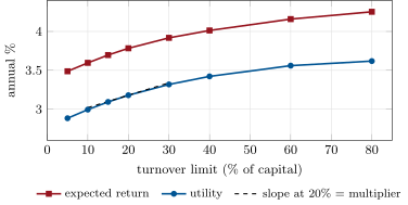
On the chapter’s portfolio (Figure 23.1), the objective is expected return minus five times the variance (annual units, covariance of chapter 22). With a 20% turnover limit the optimum has an expected return of 3.78%, a volatility of 3.47% and a utility of 3.18%; the limit binds, and its multiplier is 0.0159: each extra 1% of turnover allowed is worth 1.6 basis points of utility. Solving again with the limit at 10%, 15%, 30% and 40% traces the curve whose slope the multiplier is: 0.0210 at 10%, 0.0184 at 15%, 0.0119 at 30%, falling to 0.0011 at 80% as the limit stops mattering.

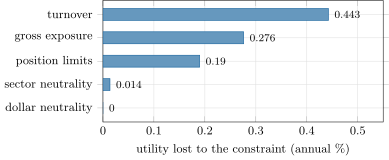
**Figure 23.1.** The price of turnover: the optimal long-short portfolio’s utility and expected return as the turnover limit is relaxed from 5% to 80% of capital. The dashed line through the 20% point has the slope of the turnover constraint’s multiplier, 0.0159 (1.6 basis points of utility per 1% of turnover). Data: the chapter’s tutorial, seeded.

Relaxing each constraint group in turn and re-solving ranks them by what they cost (Figure 23.2): the turnover limit 0.44% of utility, the gross limit 0.28%, the forty-three binding position limits together 0.19%, sector neutrality 0.014%, dollar neutrality nothing. The last is instructive: dollar neutrality is implied by the five sector neutralities, which sum to it, so it is redundant, and its multiplier (0.0004 in the solver’s answer) is not unique; a zero relaxation value with a nonzero multiplier is the signature of a redundant constraint.

**Figure 23.2.** What each constraint group costs the long-short portfolio: the gain in utility when it is removed and the problem re-solved. Dollar neutrality costs nothing because the sector neutralities imply it. Data: the chapter’s tutorial, seeded.

Definition 23.6 (Infeasibility certificate)

An infeasibility certificate for the linear system $Ax = b$ , $Gx \le h$ is a pair $(\lambda \ge 0, \nu)$ with $G^\top\lambda + A^\top\nu = 0$ and $h^\top\lambda + b^\top\nu < 0$ .

By Farkas’ lemma a certificate exists if and only if the system is infeasible: combining the rows with the weights $\lambda$ and $\nu$ gives $0 = (\lambda^\top G + \nu^\top A)x \le h^\top\lambda + b^\top\nu < 0$ , an impossibility anyone can verify. A phase-one problem, minimise $t$ subject to $Ax = b$ , $Gx \le h + t\mathbf 1$ , produces one from its dual variables when its optimum is positive. When a risk manager demands that each of the forty stocks of the first sector be held at least 0.5% long, while sector neutrality is on, the phase-one optimum is $t^* = 0.005$ and the certificate puts weight $1/40$ on each of the forty minimum-position rows and a multiplier on the first sector’s neutrality equation, and nothing on any other limit: adding the forty rows gives “the sector is at least 20% long”, and the neutrality row says it is exactly 0. The report names the two rules that clash.

23.3 Optimality conditions

Definition 23.7 (Karush–Kuhn–Tucker conditions)

The Karush–Kuhn–Tucker conditions at $(x, \lambda, \nu)$ are primal feasibility, dual feasibility ( $\lambda \ge 0$ ), complementary slackness ( $\lambda_ig_i(x) = 0$ ) and stationarity, $\nabla f(x) + \sum_i\lambda_i\nabla g_i(x) + A^\top\nu = 0$ (Karush, 1939; Kuhn and Tucker, 1951).

Theorem 23.8 (KKT conditions characterise the optimum)

For a convex problem with differentiable functions satisfying Slater’s condition, $x$ is optimal if and only if there are $(\lambda, \nu)$ such that $(x, \lambda, \nu)$ satisfies the KKT conditions; the $(\lambda, \nu)$ are then optimal dual variables.

Proof. Sufficiency: stationarity says $x$ minimises the convex function $L(\cdot, \lambda, \nu)$ , so $d(\lambda, \nu) = L(x, \lambda, \nu) = f(x)$ by complementary slackness and feasibility; weak duality then makes $x$ primal optimal and $(\lambda, \nu)$ dual optimal. Necessity: under Slater, strong duality holds with an optimal $(\lambda, \nu)$ , and $f(x) = d(\lambda, \nu) \le L(x, \lambda, \nu) \le f(x)$ forces complementary slackness and the minimisation of $L$ at $x$ , whose first-order condition is stationarity. ∎

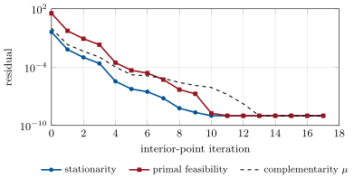
Complementary slackness is the economics: a limit that does not bind has a zero price, and a limit with a positive price binds. The solver’s answer for the portfolio satisfies the conditions to working precision: stationarity residual and complementarity both below $10^{-9}$ . The forty-three positions at the 1.5% limit carry positive multipliers, about 0.0175 each; the other 157 carry zero.

23.4 Quadratic and second-order cone programmes

Definition 23.9 (Linear, quadratic, second-order cone and semidefinite programmes)

A linear programme minimises a linear function subject to linear constraints; a quadratic programme has a convex quadratic objective and linear constraints; a second-order cone programme (SOCP) adds constraints $\lVert A_ix + b_i\rVert_2 \le c_i^\top x + d_i$ ; a semidefinite programme constrains a symmetric matrix depending affinely on $x$ to be positive semidefinite.

Each class contains the previous one. Gross exposure and turnover, sums of absolute values, become linear by splitting each position into a positive and a negative part: the chapter’s portfolio of 200 stocks is a quadratic programme in 1 000 variables.

Proposition 23.10 (Risk and impact as cone constraints)

A volatility or tracking-error limit $\sqrt{(w - b)^\top\Sigma(w - b)} \le \sigma_{\max}$ is the second-order cone constraint $\lVert L^\top(w - b)\rVert_2 \le \sigma_{\max}$ with $\Sigma = LL^\top$ . A market-impact cost growing like the 3/2 power of the traded amount, $|x|^{3/2} \le s$ , is representable with two rotated cone constraints: it holds if and only if there is $r \ge 0$ with $x^2 \le rs$ and $r^2 \le |x|$ .

Proof. The first is the identity $w^\top\Sigma w = \lVert L^\top w\rVert^2$ . For the second (with $x \ge 0$ after splitting), if $x^{3/2} \le s$ take $r = \sqrt x$ : then $r^2 = x$ and $x^2 = \sqrt x\,x^{3/2} \le rs$ . Conversely $r^2 \le x$ gives $r \le \sqrt x$ , so $x^2 \le rs \le \sqrt x\,s$ and $x^{3/2} \le s$ . Each constraint $u^2 \le vw$ with $v, w \ge 0$ is a rotated second-order cone, $\lVert(2u, v - w)\rVert \le v + w$ . ∎

A risk limit and a risk penalty are the same problem seen from two sides. Maximising expected return subject to a 4% volatility limit (dollar-neutral, positions within 1.5%) by the firm’s cone solver, and maximising return minus $\gamma/2$ times variance with $\gamma$ found by bisection to give 4% volatility, produce the same portfolio (the weights differ by $3 \times 10^{-8}$ ), an expected return of 5.31%, $\gamma = 25.8$ , and a cone multiplier of 1.033 $= \gamma \times 0.04$ : the shadow price of the volatility limit, expected return per unit of volatility allowed.

Definition 23.11 (Nearest correlation matrix)

The nearest correlation matrix to a symmetric matrix $C$ is the positive semidefinite matrix with unit diagonal closest to $C$ in the Frobenius norm, a semidefinite programme that Higham (2002) solves by alternating projections with Dykstra’s correction.

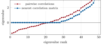
Correlations estimated pair by pair from data with gaps are not guaranteed to form a correlation matrix, and a covariance built from them can make an optimiser promise negative variance. Fifty series of sixty days with half the observations missing give a pairwise matrix with 21 negative eigenvalues, the smallest $-1.42$ ; the nearest correlation matrix, reached in 74 projections, is 4.45 away in the Frobenius norm, changes no entry by more than 0.31, and has no negative eigenvalue (Figure 23.3).

**Figure 23.3.** Eigenvalues (in increasing order; the largest, above 10, off the chart) of a pairwise-complete correlation matrix of fifty series with half the data missing, and of its nearest correlation matrix. Twenty-one negative eigenvalues become zero. Data: the chapter’s tutorial, seeded.

23.5 What solvers actually do

Definition 23.12 (Interior-point method)

An interior-point method follows the central path: it applies Newton’s method to the KKT conditions with complementary slackness relaxed to $s_iz_i = \mu$ for slacks $s$ and multipliers $z$ , keeping both strictly positive, and drives $\mu$ to zero.

Each iteration solves one linear system in the Newton direction; Mehrotra’s (1992) predictor-corrector computes an affine direction, uses it to choose how far to reduce $\mu$ , and corrects for the second-order term, with the same matrix factorisation. The number of iterations barely depends on the problem’s size: the chapter’s portfolio converges in 18, the residuals and the complementarity falling from order one to below $10^{-9}$ (Figure 23.4). Interior-point methods descend from Karmarkar’s (1984) polynomial algorithm for linear programmes and were extended to cone programmes by Nesterov and Nemirovskii (1994). First-order splitting methods such as ADMM, of which the OSQP solver (Stellato and coauthors, 2020) is a production example, need only one factorisation and cheap iterations, reach moderate accuracy fast, and warm-start well when yesterday’s solution is close to today’s; the firm’s cone solver is of this kind, and needed 924 iterations for the 4% volatility limit above.

Convergence of the firm’s interior-point solver on the long-short portfolio (1 000 variables): the norms of the stationarity and feasibility residuals and the average complementarity at each Mehrotra iteration, floored at 10-9 (below it, the last digits depend on the order of floating-point operations). Data: the chapter’s tutorial, seeded. — **Figure 23.4.** Convergence of the firm’s interior-point solver on the long-short portfolio (1 000 variables): the norms of the stationarity and feasibility residuals and the average complementarity $\mu$ at each Mehrotra iteration, floored at $10^{-9}$ (below it, the last digits depend on the order of floating-point operations). Data: the chapter’s tutorial, seeded.

23.6 Tutorial: the constraint that cost the most

Goal. Formulate the long-short portfolio as a quadratic programme, solve it with the firm’s interior-point method, verify the KKT conditions, read the shadow prices, and read the certificate of an infeasible set of limits. End state: Figures 23.1, 23.2 and 23.4; the turnover multiplier 0.0159 and the ranking of the constraints.

The Newton step of the interior-point method, with the predictor and the corrector sharing one matrix.

def qp(P, q, A=None, b=None, G=None, h=None, tol: float = 1e-9, max_iter: int = 100) -> dict:
    P = np.atleast_2d(np.asarray(P, dtype=float))
    q = np.asarray(q, dtype=float)
    n = q.size
    A = np.zeros((0, n)) if A is None else np.atleast_2d(np.asarray(A, dtype=float))
    b = np.zeros(0) if b is None else np.asarray(b, dtype=float)
    G = np.zeros((0, n)) if G is None else np.atleast_2d(np.asarray(G, dtype=float))
    h = np.zeros(0) if h is None else np.asarray(h, dtype=float)
    m, p = G.shape[0], A.shape[0]
    x, y = np.zeros(n), np.zeros(p)
    s, z = np.ones(m), np.ones(m)
    history = []
    status = "max_iter"
    scale = 1 + max(np.abs(q).max(initial=0), np.abs(h).max(initial=0), np.abs(b).max(initial=0))
    for it in range(max_iter):
        rd, rp, ri = _kkt_residuals(P, q, A, b, G, h, x, y, z, s)
        mu = float(s @ z) / m if m else 0.0
        feas = float(np.linalg.norm(np.concatenate([rp, ri])))
        history.append((it, float(np.linalg.norm(rd)), feas, mu))
        if np.linalg.norm(rd) < tol * scale and feas < tol * scale and mu < 1e-3 * tol:
            status = "optimal"
            break
        Hm = P + G.T @ (G * (z / s)[:, None])
        K = np.block([[Hm, A.T], [A, np.zeros((p, p))]]) if p else Hm
        K = K + 1e-12 * np.eye(K.shape[0])
        dx, dy, ds, dz = _newton(K, G, n, p, rd, rp, ri, s, z, s * z)                   # affine (predictor)
        a = min(_step_len(s, ds), _step_len(z, dz)) if m else 1.0
        mu_aff = float((s + a * ds) @ (z + a * dz)) / m if m else 0.0
        sigma = (mu_aff / mu) ** 3 if m and mu > 0 else 0.0
        dx, dy, ds, dz = _newton(K, G, n, p, rd, rp, ri, s, z, s * z + ds * dz - sigma * mu)  # corrector
        a = 0.99 * min(_step_len(s, ds), _step_len(z, dz)) if m else 1.0
        x, y, s, z = x + a * dx, y + a * dy, s + a * ds, z + a * dz

Listing 23.1. The interior-point iteration: Mehrotra’s predictor and corrector share one matrix. code/firm/portopt/firm_portopt.py

The phase-one problem and its Farkas certificate.

def farkas(A, b, G, h, tol: float = 1e-7):
    """Phase one: minimise t subject to Ax = b, Gx <= h + t. If the optimum t* > 0 the system is infeasible, and the
    duals (lam, nu) satisfy G'lam + A'nu = 0, sum(lam) = 1, h'lam + b'nu = -t* < 0: a Farkas certificate."""
    A, G = np.atleast_2d(np.asarray(A, float)), np.atleast_2d(np.asarray(G, float))
    b, h = np.asarray(b, float), np.asarray(h, float)
    n, m = G.shape[1], G.shape[0]
    Gt = np.hstack([G, -np.ones((m, 1))])
    At = np.hstack([A, np.zeros((A.shape[0], 1))])
    q = np.zeros(n + 1)
    q[-1] = 1.0
    P = 1e-10 * np.eye(n + 1)                          # a whisper of curvature keeps the KKT matrix regular
    t_box = np.zeros(n + 1)
    t_box[-1] = -1.0                                                    # t >= -1 keeps the phase-one problem bounded
    sol = qp(P, q, At, b, np.vstack([Gt, t_box]), np.concatenate([h, [1.0]]), tol=1e-10)
    t = sol["x"][-1]
    if t <= tol:
        return None
    lam, nu = sol["z"][:m], sol["y"]
    return lam, nu, float(t)

Listing 23.2. Phase one and the infeasibility certificate. code/firm/portopt/firm_portopt.py

Run today(), constraint_costs(), turnover_curve(), infeasible(), risk_limit() and broken_correlation() in qm_opt.py, then fig_opt.py.

What to change next. Replace the turnover limit by a 3/2-power impact cost in the objective and compare the traded amounts; warm-start the interior-point method from yesterday’s solution and count the iterations saved.

23.7 Build: the portfolio optimiser

Purpose. The miniature firm’s portfolio construction: forecasts, a covariance (chapter 22) and the limits in, orders out, with a price for each limit and a certificate when the limits contradict each other.

Interface. qp(P, q, A, b, G, h); farkas(A, b, G, h); admm(P, q, C, lower, upper, cones); PortfolioProblem(alpha, Sigma, gamma, w0) with add_budget, add_neutral, add_box, add_gross, add_turnover and solve(); nearest_correlation(C).

Rules. Every solve reports its status, KKT residuals and the dual variable of each named constraint; an infeasible request returns the certificate, never a silently relaxed portfolio; covariances pass a positive-semidefiniteness check (and the nearest-correlation repair) before use.

Acceptance tests. code/firm/portopt/tests/: a small QP and its KKT residuals; the minimum-variance closed form and its multiplier; Farkas certificates on feasible and infeasible systems; the cone solver on a norm ball; portfolio constraints hold and the turnover multiplier equals the finite-difference slope; the nearest correlation matrix is a correlation matrix and leaves one unchanged.

Stretch. A homogeneous self-dual embedding (certificates without phase one); sparse KKT factorisation for thousands of assets; the 3/2-power impact cost in the cone solver.

Sources and further reading

W. Karush, Minima of Functions of Several Variables with Inequalities as Side Constraints, MSc thesis, University of Chicago, 1939; H. W. Kuhn and A. W. Tucker, “Nonlinear programming”, Second Berkeley Symposium, 1951.
H. Markowitz, “Portfolio selection”, Journal of Finance 7, 1952.
N. Karmarkar, “A new polynomial-time algorithm for linear programming”, Combinatorica 4, 1984; S. Mehrotra, “On the implementation of a primal-dual interior point method”, SIAM Journal on Optimization 2, 1992.
Y. Nesterov and A. Nemirovskii, Interior-Point Polynomial Algorithms in Convex Programming, SIAM, 1994.
S. Boyd and L. Vandenberghe, Convex Optimization, Cambridge University Press, 2004.
M. S. Lobo, L. Vandenberghe, S. Boyd and H. Lebret, “Applications of second-order cone programming”, Linear Algebra and its Applications 284, 1998.
N. J. Higham, “Computing the nearest correlation matrix: a problem from finance”, IMA Journal of Numerical Analysis 22, 2002.
B. Stellato, G. Banjac, P. Goulart, A. Bemporad and S. Boyd, “OSQP: an operator splitting solver for quadratic programs”, Mathematical Programming Computation 12, 2020.

23.8 Exercises

Exercise 23.1 ★

Is $f(w) = \sqrt{w^\top\Sigma w}$ convex for positive semidefinite $\Sigma$ ? Is $\{w: w^\top\Sigma w \ge 0.01\}$ a convex set?

Solution

Solution of Exercise 23.1.

Yes: $\sqrt{w^\top\Sigma w} = \lVert L^\top w\rVert$ is a norm composed with a linear map, hence convex. No: the set where the variance is at least a level is the complement of an ellipsoid; the segment between $w$ and $-w$ passes through $0$ , where the variance is zero.

Exercise 23.2 ★

The turnover multiplier is 0.0159. Estimate the utility gained by raising the limit from 20% to 22%, and compare with re-solving (the curve gives 3.180% at 20% and a slope of 0.0139 over [20%, 30%]).

Solution

Solution of Exercise 23.2.

First order: $0.0159 \times 0.02 = 0.032\%$ , so about $3.180\% + 0.032\% = 3.212\%$ . Re-solving at 22% gives 3.211%: the multiplier slightly overstates the gain because the price falls as the limit loosens.

Exercise 23.3 ★

Write $\sum_i|w_i - w_{0,i}| \le \tau$ with linear constraints only.

Solution

Solution of Exercise 23.3.

Introduce $u, v \ge 0$ with $w - w_0 = u - v$ and require $\mathbf 1^\top(u + v) \le \tau$ . At the optimum $u_iv_i = 0$ for every $i$ whenever the limit binds, so $u + v = |w - w_0|$ .

Exercise 23.4 ★★

Derive the minimum-variance portfolio and its multiplier from the KKT conditions of $\min\frac12w^\top\Sigma w$ subject to $\mathbf 1^\top w = 1$ .

Solution

Solution of Exercise 23.4.

Stationarity $\Sigma w + \nu\mathbf 1 = 0$ gives $w = -\nu\Sigma^{-1}\mathbf 1$ ; the budget gives $\nu = -1/(\mathbf 1^\top\Sigma^{-1}\mathbf 1)$ , so $w = \Sigma^{-1}\mathbf 1/(\mathbf 1^\top\Sigma^{-1}\mathbf 1)$ . The multiplier’s magnitude is the minimum variance, $1/(\mathbf 1^\top\Sigma^{-1}\mathbf 1)$ : the rate at which the (half) variance grows with the budget.

Exercise 23.5 ★★

Find a Farkas certificate for $x_1 + x_2 = 1$ , $x_1 \le 0.2$ , $x_2 \le 0.3$ .

Solution

Solution of Exercise 23.5.

$\lambda = (1, 1)$ on the two upper bounds and $\nu = -1$ on the equation: $G^\top\lambda + A^\top\nu = (1, 1) - (1, 1) = 0$ and $h^\top\lambda + b^\top\nu = 0.5 - 1 = -0.5 < 0$ . In words: $x_1 + x_2 \le 0.5$ contradicts $x_1 + x_2 = 1$ .

Exercise 23.6 ★★

Show that $\max\alpha^\top w$ subject to $w^\top\Sigma w \le \sigma^2$ (no other constraint) has solution $w = \sigma\Sigma^{-1}\alpha/\sqrt{\alpha^\top\Sigma^{-1}\alpha}$ and a shadow price of the volatility limit equal to $\sqrt{\alpha^\top\Sigma^{-1}\alpha}$ .

Solution

Solution of Exercise 23.6.

KKT: $\alpha = 2\lambda\Sigma w$ , so $w \propto \Sigma^{-1}\alpha$ ; the binding limit fixes the scale, $w = \sigma\Sigma^{-1}\alpha/\sqrt{\alpha^\top\Sigma^{-1}\alpha}$ , and the optimal value is $\sigma\sqrt{\alpha^\top\Sigma^{-1}\alpha}$ , whose derivative in $\sigma$ is $\sqrt{\alpha^\top\Sigma^{-1}\alpha}$ , the maximal Sharpe ratio: the shadow price of the volatility limit.

Exercise 23.7 ★★★

Coding. Rank the constraint groups of the chapter’s portfolio by the utility each costs, by relaxing them one at a time, and explain the result for dollar neutrality.

Solution

Solution of Exercise 23.7.

constraint_costs(): turnover 0.44% of utility, gross exposure 0.28%, position limits 0.19%, sector neutrality 0.014%, dollar neutrality 0. The dollar constraint is the sum of the five sector constraints, so removing it changes nothing; its multiplier in the solver’s answer is not unique and says nothing.

Exercise 23.8 ★★★

Find the flaw. “The optimiser failed tonight, so the overnight job dropped constraints one at a time until it found a feasible portfolio, and traded that.”

Solution

Solution of Exercise 23.8.

Dropping constraints in an arbitrary order trades a portfolio that violates a limit chosen by the order of the code, not by anyone’s judgement, and hides the conflict. Compute the infeasibility certificate, report the conflicting rules to the people who own them, and trade nothing new (or a documented fallback) until a limit is changed deliberately.

23.9 Problem: The Constraint That Cost the Most

Problem 23.1

Weekend problem — pricing the limits of a long-short book

A book of 200 stocks (the factor covariance of chapter 22, annual units) maximises expected return minus five times the variance, dollar- and sector-neutral, positions within 1.5%, gross exposure at most 100%, turnover at most 20% against yesterday’s optimal book. Today’s forecasts are yesterday’s decayed by 0.8 plus news.

Part I — The optimum.

What are the optimal portfolio’s expected return, volatility and utility?
Which constraints bind, and how many positions sit at their limits?
How many interior-point iterations does the solver need, and what are the KKT residuals?
What is the turnover limit’s multiplier, and what does it mean?
What is the gross-exposure multiplier?

Part II — Prices.

How does the utility change as the turnover limit goes from 5% to 80%?
How do the multipliers compare with the slopes of that curve?
Rank the constraint groups by the utility each costs.
Why is the dollar-neutrality cost zero although its multiplier is not?
What is the expected return given up per 1% of turnover?

Part III — When there is no portfolio.

What happens when sector 0’s stocks must each be at least 0.5% long?
What does the certificate say, and how is it checked?
How would a volatility limit of 4% be expressed, and what is its shadow price?
Why must the correlation matrix be checked before optimising?
What does the nearest correlation matrix do to a pairwise matrix with 21 negative eigenvalues?

Part IV — Judgement.

Which limit would you ask the risk committee to loosen first?
Is a 1.6-basis-point price per 1% of turnover worth paying, and against what?
What should the optimiser’s report contain every day?
State the named result: the shadow price of the turnover limit and the ranking of the constraints by the return they cost.
In one sentence: what does duality give a portfolio manager that the solution alone does not?

Solution

Solution of Problem 23.1.

1. Expected return 3.78%, volatility 3.47%, utility 3.18% (annual). 2. Gross exposure (100%), turnover (20%), 43 position limits; the neutralities hold as equations. 3. 18 iterations; stationarity and complementarity residuals below $10^{-9}$ . 4. 0.0159: one more percent of turnover is worth 1.6 basis points of utility. 5. 0.0185 per unit of gross exposure. 6. From 2.88% at 5% to 3.18% at 20% and 3.62% at 80%. 7. They are the slopes: 0.0210, 0.0184, 0.0159, 0.0119 and 0.0011 at 10%, 15%, 20%, 30% and 80%, matching the finite differences of the curve. 8. Turnover 0.44%, gross 0.28%, positions 0.19%, sector neutrality 0.014%, dollar neutrality 0. 9. It is implied by the sector neutralities (their sum), so it is redundant; multipliers of redundant constraints are not unique. 10. Expected return rises from 3.60% to 3.92% between 10% and 30% turnover: 1.6 basis points per 1% of turnover, close to the utility price. 11. The limits are infeasible: phase one ends at $t^* = 0.005$ . 12. Weights $1/40$ on each minimum-position row of sector 0 and a multiplier on the sector’s neutrality equation; adding the rows gives “sector 0 at least 20% long” against “sector 0 exactly 0”: the combination $G^\top\lambda + A^\top\nu = 0$ with $h^\top\lambda + b^\top\nu = -0.005 < 0$ . 13. As the cone constraint $\lVert L^\top w\rVert \le 0.04$ ; its shadow price is 1.033 ( $= \gamma \times 0.04$ with $\gamma = 25.8$ ), expected return per unit of volatility allowed; the portfolio earns 5.31%. 14. A matrix with negative eigenvalues makes some portfolios’ variance negative, and the optimiser will find and exploit them. 15. In 74 projections it removes all 21 negative eigenvalues at a Frobenius distance of 4.45, changing no entry by more than 0.31. 16. Turnover: it costs the most (0.44% of utility), and its price is 1.6 basis points per 1% traded. 17. Only against the transaction costs the limit is there to save: if trading 1% of capital costs less than 1.6 basis points, the limit is too tight; the limit is a proxy for a cost model that should be in the objective. 18. Status, KKT residuals, the value of each binding constraint and its multiplier, the ranking by relaxation, and any certificate. 19. Named result: the constraint that cost the most: the turnover limit’s shadow price is 0.0159, 1.6 basis points of utility per 1% of turnover, and the constraints rank turnover (0.44%), gross exposure (0.28%), position limits (0.19%), sector neutrality (0.014%), dollar neutrality (redundant, 0). 20. It prices every limit in the units of the objective, so limits can be argued about with numbers, and it proves infeasibility when there is nothing to trade.

23.10 Interview questions

Interview question 23.1 ★ researcher, developer

Why is convexity so important in optimisation?

Solution

Solution of Interview question 23.1.

Because every local optimum is global, so a solver that satisfies local optimality conditions has the answer, and those conditions (KKT) can be checked; duality then gives bounds, prices and infeasibility certificates, and polynomial-time algorithms exist.

What the interviewer is looking for: Local equals global, checkable optimality, and duality.

Interview question 23.2 ★★ researcher, trader

What is a shadow price, and how would you use one to argue for loosening a risk limit?

Solution

Solution of Interview question 23.2.

The optimal dual variable of a constraint: the rate at which the optimal objective improves per unit of relaxation. Show the committee the multiplier of the risk or turnover limit in return per unit, compare it with what the limit protects against (cost, risk), and confirm by re-solving with the limit relaxed.

What the interviewer is looking for: Marginal value in objective units, and confirmation by relaxation.

Interview question 23.3 ★★ researcher

State the KKT conditions and explain complementary slackness in portfolio terms.

Solution

Solution of Interview question 23.3.

Feasibility of the primal and of the dual ( $\lambda \ge 0$ ), stationarity of the Lagrangian, and $\lambda_ig_i(x) = 0$ . In a portfolio: a limit that does not bind has zero price, and a limit with a positive price is exactly at its bound; positions strictly inside their limits have a marginal utility equal to the prices of the binding constraints they touch.

What the interviewer is looking for: All four conditions and the economic reading of complementarity.

Interview question 23.4 ★★ developer, researcher

Your optimiser says a problem is infeasible. How do you find out which constraints conflict?

Solution

Solution of Interview question 23.4.

Solve a phase-one (or self-dual) problem and read the Farkas certificate: the constraints with positive weight form a conflicting subset, which can be reported to their owners. Alternatively minimise the total violation with weights reflecting priorities.

What the interviewer is looking for: Certificates rather than trial and error.

Interview question 23.5 ★★ developer

Interior-point or first-order methods for a daily portfolio rebalance of 3 000 stocks: which, and why?

Solution

Solution of Interview question 23.5.

Interior-point methods give high accuracy in a few dozen iterations whatever the size, with exploitable structure (factor covariance) in the linear algebra; first-order methods such as ADMM have cheap iterations, warm-start well from yesterday’s solution and reach trading accuracy quickly. For a daily rebalance with a factor model either works; ADMM with warm starts is attractive intraday, interior points when duals must be accurate.

What the interviewer is looking for: Accuracy versus warm starts, and exploiting the factor structure.

Interview question 23.6 ★★★ researcher

How do you write a tracking-error limit and a 3/2-power impact cost as convex constraints?

Solution

Solution of Interview question 23.6.

Tracking error: $\lVert L^\top(w - b)\rVert_2 \le \mathrm{TE}$ with $\Sigma = LL^\top$ , a second-order cone. Impact $|x|^{3/2} \le s$ : split $x$ into positive parts and require $x^2 \le rs$ and $r^2 \le x$ with $r \ge 0$ , two rotated cones; sum the $s$ in the objective.

What the interviewer is looking for: The Cholesky trick and the power-cone decomposition.

Terms defined in this chapter

See all 2333 terms in the glossary