21High-Frequency Econometrics

Measured from one-second changes in the last traded price, a stock’s annualised volatility is 60%; from five-minute changes it is 25%. The difference is not the market’s. The trades alternate between the bid and the ask, and the prices sit on a one-cent grid; at one second those two effects are most of the measured variation, and at five minutes almost none of it. Chapter 18 promised that realised variance converges to the true integrated variance as the sampling gets finer; this chapter is about why, in real prices, it does the opposite, and what to do about it: the noise and the signature plot that reveals it, the optimal sampling interval, estimators that remove the noise instead of avoiding it, the correlation that vanishes when two assets trade at different moments, and jumps.

The chapter’s market is simulated, so that every estimate can be checked against the truth: an efficient log price with 25% annual volatility, around 36 dollars, traded once a second at the bid or the ask of a one-cent grid (the bid is the efficient price rounded down to the cent, the ask one cent higher), over 6.5-hour days of 23 400 seconds.

21.1 Microstructure noise and the signature plot

Definition 21.1 (Microstructure noise, bid–ask bounce)

Microstructure noise is the difference between an observed price and the efficient price, created by the trading process: the spread, the price grid, the discreteness and staleness of quotes. The bid–ask bounce is its best-known form: successive trades at the bid and at the ask make observed returns alternate in sign when the efficient price has not moved.

If the observed log price is $Y_i = X_i + u_i$ with iid noise $u_i$ of variance $\omega^2$ independent of the efficient $X$, each observed return carries $u_i - u_{i-1}$, so realised variance from $n$ returns has

a bias that grows linearly with the sampling frequency and swamps the integrated variance at high frequency. The noise also makes consecutive returns negatively correlated, with first autocovariance $-\omega^2$.

Definition 21.2 (Roll’s estimator)

Roll’s estimator (Roll, 1984) of the effective bid–ask spread is $2\sqrt{-\gamma_1}$, with $\gamma_1$ the first autocovariance of trade-price changes: under pure bounce around an efficient price, trades are at mid $\pm c/2$ with independent signs, and $\gamma_1 = -c^2/4$.

On the simulated stock, whose spread is one cent, Roll’s estimator averages 1.14 cents over thirty days: close, and biased up because the efficient price also moves the bid within the grid.

Definition 21.3 (Signature plot)

A signature plot draws average realised volatility against the sampling interval: flat without noise, rising toward the shortest intervals with it (Andersen, Bollerslev, Diebold and Labys, 2000, who named it the volatility signature plot).

Figure 21.1 is the chapter’s signature plot. From trades, realised volatility is 60.1% at one second, 35.1% at five seconds, 26.1% at one minute and 25.4% at five minutes; from mid quotes, which do not bounce but still sit on the grid, 36.8% at one second; from the efficient price, 25.0% at every interval.

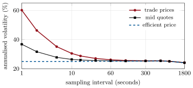
The noise variance can be estimated from the highest frequency itself, $\hat\omega^2 = \mathrm{RV}_n/(2n)$ (which also counts $\mathrm{IV}/2n$, negligible here): 1.75 basis points of standard deviation, against the true 1.60. Sampling less often trades bias for variance, and the trade has an optimum.

Proposition 21.4 (Optimal sampling under iid noise)

With iid noise of variance $\omega^2$ and constant volatility, the mean squared error of $\mathrm{RV}_n$ is approximately $2\,\mathrm{IQ}/n + (2n\omega^2)^2$, where $\mathrm{IQ} = \int\sigma^4$ is the integrated quarticity; it is minimised at $n^* = (\mathrm{IQ}/(4\omega^4))^{1/3}$ (Bandi and Russell, 2008).

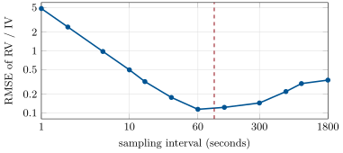
With the estimated noise, the noise-to-signal ratio $\omega^2/\mathrm{IV}$ is $1.24 \times 10^{-4}$ and $n^* = 254$ returns a day, one every 92 seconds (82 with the true noise). The simulation agrees: the root-mean-squared relative error of daily realised variance is 4.80 at one second, 0.18 at 30 seconds, 0.11 at 60, 0.12 at 120 and 0.14 at five minutes (Figure 21.2). One-second sampling overstates the variance 5.8-fold; the optimum avoids that bias at the cost of using a fraction of the data.

21.2 Estimators robust to noise

Sparse sampling throws away most of the data. Three families use it all and remove the noise.

Definition 21.5 (Two-scales realised variance)

The two-scales realised variance (Zhang, Mykland and Aït-Sahalia, 2005) averages the realised variances of the $K$ offset sparse grids and subtracts the noise bias estimated from the full grid: $\mathrm{TSRV} = \overline{\mathrm{RV}}^{(K)} - (\bar n/n)\mathrm{RV}^{(\mathrm{all})}$, $\bar n = (n - K + 1)/K$.

Averaging over the $K$ grids reduces the discretisation error of the sparse estimator; the subtraction removes its remaining bias $2\bar n\omega^2$. It is consistent under iid noise, at the slow rate $n^{-1/6}$.

Definition 21.6 (Realised kernel, pre-averaging estimator)

A realised kernel (Barndorff-Nielsen, Hansen, Lunde and Shephard, 2008) adds weighted autocovariances of the high-frequency returns to their variance, $\gamma_0 + \sum_{h=1}^Hk\bigl(\frac{h-1}H\bigr)(\gamma_h + \gamma_{-h})$, with a smooth weight such as Parzen’s, to cancel the negative autocovariance the noise creates. The pre-averaging estimator (Jacod, Li, Mykland, Podolskij and Vetter, 2009) averages returns over short overlapping windows with a weight function, which shrinks the noise in each window, then squares and rescales the averages and subtracts the remaining bias.

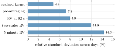
The kernel is the long-run variance of chapter 11 applied within a day: the noise makes high-frequency returns an MA(1), and a HAC-type sum recovers the variance of the efficient part. Over thirty simulated days, the average annualised volatility from trades is 25.4% by five-minute RV, 25.2% by two-scales RV ($K = 300$), 25.8% by RV at the optimal interval, 25.1% by pre-averaging (windows of 150 seconds) and 25.1% by the realised kernel ($H = 60$). The day-to-day relative standard deviations separate them (Figure 21.3): 14.3% for five-minute RV, 11.9% for two-scales, 7.9% at the optimal interval, 7.2% for pre-averaging and 4.8% for the kernel.

21.3 Asynchronous observation and the Epps effect

Definition 21.7 (Non-synchronous trading, Epps effect)

Non-synchronous trading is the observation of different assets at different, random times. The Epps effect (Epps, 1979) is the resulting fall of realised correlation toward zero as the sampling interval shortens: with previous-tick sampling on a fine grid, most intervals contain a price change of one asset and none of the other.

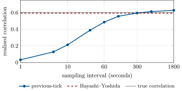
Two simulated stocks with a true correlation of 0.6, trading at Poisson times every 5 and every 15 seconds on average, show it cleanly (Figure 21.4): realised correlation from previous-tick prices is 0.03 at one second, 0.21 at ten seconds, 0.49 at one minute, 0.59 at five minutes and 0.63 at thirty minutes (where the sampling error of few returns takes over).

Definition 21.8 (Hayashi–Yoshida estimator, refresh-time sampling)

The Hayashi–Yoshida estimator (Hayashi and Yoshida, 2005) of the covariation sums the products of all pairs of returns, one from each asset, whose observation intervals overlap, with no interpolation. Refresh-time sampling samples both assets at the first time each has traded since the previous sampling time.

The Hayashi–Yoshida estimator is unbiased for the covariation of the efficient prices without noise, whatever the observation times, because every piece of the covariance is counted once. On the two stocks it gives an average correlation of 0.594 (true 0.6), with a day-to-day standard deviation of 0.030. Refresh-time sampling alone gives 0.48: it synchronises the sampling, but the last prices it pairs were still observed at different moments.

21.4 Jumps at high frequency

Definition 21.9 (Bipower variation)

Bipower variation (Barndorff-Nielsen and Shephard, 2004) is $\frac\pi2\sum_i|r_i||r_{i-1}|$: products of adjacent absolute returns, scaled by $1/\E|Z|^2 = \pi/2$.

Realised variance converges to the whole quadratic variation, the integrated variance plus the sum of squared jumps; bipower variation converges to the integrated variance alone, because a jump enters only through products with a neighbouring, diffusive return, which vanish as the sampling gets finer. The difference estimates the jump part. At five-minute sampling, over forty simulated days with a 1% jump at midday (29% of that day’s quadratic variation), realised variance averages 1.43 times the integrated variance and bipower variation 1.16; without the jump, 1.00 and 1.00. At five minutes the jump still leaks into bipower variation through its two neighbouring products; the cure is finer sampling, which brings back the noise, and so jump detection and noise-robust estimation have to be combined in practice.

21.5 Tutorial: the volatility that depended on the clock

21.6 Build: the high-frequency estimators

21.7 Exercises

Exercise 21.1 ★

A stock’s daily integrated variance is $(1\%)^2$ and its iid noise has a standard deviation of 2 basis points. What is the expected realised variance from 23 400 one-second returns, and the implied daily volatility?

Solution

Solution of Exercise 21.1.

$\E[\mathrm{RV}] = 10^{-4} + 2 \times 23\,400 \times (2 \times 10^{-4})^2 = 10^{-4} + 1.87 \times 10^{-3} = 1.97 \times 10^{-3}$: a daily volatility of 4.4% for a true 1%.

Exercise 21.2 ★

Trade-price changes have first autocovariance $-0.0004$ (dollars squared). What spread does Roll’s estimator imply?

Solution

Solution of Exercise 21.2.

$2\sqrt{0.0004} = 0.04$ dollars, four cents.

Exercise 21.3 ★

Why do mid quotes show less noise than trade prices in the signature plot, but still some?

Solution

Solution of Exercise 21.3.

The mid does not jump between bid and ask with the trade sign, so the bounce is gone; but it moves only when the quotes cross a grid point, so it is the efficient price rounded to half-ticks, and the rounding error is noise.

Exercise 21.4 ★★

Compute the Bandi–Russell optimal number of returns and interval for a daily volatility of 1% (constant) and noise of 2 basis points, over 23 400 seconds.

Solution

Solution of Exercise 21.4.

$\mathrm{IQ} = (10^{-4})^2 = 10^{-8}$ and $\omega^4 = (4 \times 10^{-8})^2 = 1.6 \times 10^{-15}$, so $n^* = (10^{-8}/6.4 \times 10^{-15})^{1/3} = 116$ returns, one every 202 seconds.

Exercise 21.5 ★★

Show that with iid noise, observed high-frequency returns have first autocorrelation $-\omega^2/(\sigma^2\Delta + 2\omega^2)$, and evaluate it for the chapter’s stock at one second.

Solution

Solution of Exercise 21.5.

An observed return is $r_i + u_i - u_{i-1}$ with variance $\sigma^2\Delta + 2\omega^2$; two consecutive ones share $u_{i-1}$ with opposite signs, so their covariance is $-\omega^2$. For the chapter’s stock at one second, $\sigma^2\Delta = 2.48 \times 10^{-4}/23\,400 = 1.06 \times 10^{-8}$ and $\omega^2 = 2.56 \times 10^{-8}$: $-2.56/(1.06 + 5.12) = -0.41$, as measured in the simulation ($-0.41$).

Exercise 21.6 ★★

Two assets trade on average every 5 and 15 seconds. Roughly what share of one-second intervals contains a trade in both?

Solution

Solution of Exercise 21.6.

With independent trading, $0.2 \times 1/15 = 1.3\%$ of one-second intervals contain a trade in both; in the others, at least one previous-tick return is zero, which is why the one-second correlation collapses.

Exercise 21.7 ★★★

Coding. Draw the signature plot of the simulated stock from trades, mid quotes and efficient prices, and compute the root-mean-squared error of realised variance at each interval.

Solution

Solution of Exercise 21.7.

signature() and mse_by_interval(): trades 60.1%, 35.1%, 26.1%, 25.4% at 1, 5, 60, 300 seconds; mids 36.8% at one second; efficient 25.0% everywhere. The root-mean-squared relative error is 4.80 at one second and smallest near one minute (0.11 at 60 seconds, 0.12 at 120).

Exercise 21.8 ★★★

Find the flaw. “To estimate the correlation of two stocks as precisely as possible, we used every one-second return of both over a year; the correlation is 0.12, so the pair is useless for hedging.”

Solution

Solution of Exercise 21.8.

One-second returns of two stocks rarely contain trades in both, so previous-tick realised correlation is biased toward zero (the Epps effect): 0.12 is an artefact of the sampling, not a property of the pair. Use Hayashi–Yoshida, or sample at several minutes, or a synchronised noise-robust estimator, and compare.

21.8 Problem: The Volatility That Depended on the Clock

Problem 21.1

Weekend problem — sampling a noisy price

A simulated stock has efficient volatility 25% a year, trades once a second at the bid or ask of a one-cent grid around 36 dollars, over 23 400-second days.

Part I — The signature plot.

1. What volatility do one-second, five-second, one-minute and five-minute trade returns give?
2. And mid quotes at one second? The efficient price?
3. What is the noise standard deviation, estimated and true?
4. What does Roll’s estimator say about the spread?
5. Why is the one-second variance 5.8 times too large?

Part II — The optimal interval.

6. What noise-to-signal ratio do the data imply?
7. What is the Bandi–Russell optimal number of returns and interval?
8. How does the simulated root-mean-squared error vary with the interval?
9. What does the optimum cost in data?
10. How would the optimum change on a day twice as volatile?

Part III — Beyond sampling.

11. What do two-scales RV, pre-averaging and the realised kernel give, and how precisely?
12. What is the Epps effect for two stocks trading every 5 and 15 seconds?
13. What do Hayashi–Yoshida and refresh-time sampling give?
14. What does a 1% jump do to realised and bipower variation at five minutes?
15. Why can’t jumps and noise be handled separately?

Part IV — Judgement.

16. Which intraday volatility should a market maker’s quoting engine use?
17. Which correlation should its hedging use?
18. What would you check on real data that the simulation assumes away?
19. State the named result: the optimal sampling interval and the bias of one-second realised variance it avoids.
20. In one sentence: why does more data make realised variance worse?

Solution

Solution of Problem 21.1.

1. 60.1%, 35.1%, 26.1% and 25.4%. 2. 36.8% from mid quotes at one second; 25.0% from the efficient price at every interval. 3. Estimated from $\mathrm{RV}/2n$: 1.75 basis points; true: 1.60 (a trade is uniformly within one tick of the efficient price, a tick being 2.8 basis points). 4. 1.14 cents, against a true one-cent spread. 5. Each one-second return carries a noise difference of variance $2\omega^2$, about five times the efficient variance per second, and 23 400 of them add up: RV is 5.8 times the integrated variance. 6. $\omega^2/\mathrm{IV} = 1.24 \times 10^{-4}$. 7. $n^* = 254$, one return every 92 seconds (82 with the true noise). 8. 4.80 at one second, 0.98 at five, 0.18 at thirty, 0.11 at sixty, 0.12 at 120, 0.14 at 300 and 0.34 at 1 800 seconds. 9. It uses 254 of 23 400 returns, about 1%. 10. $n^* \propto \mathrm{IQ}^{1/3}$ and IQ scales with the square of the variance, so doubling the variance multiplies $n^*$ by $2^{2/3} = 1.59$: sample about every 58 seconds. 11. 25.2%, 25.1% and 25.1%, with daily relative errors of 11.9%, 7.2% and 4.8% (five-minute RV: 25.4% and 14.3%). 12. Realised correlation 0.03 at one second, 0.21 at ten, 0.49 at sixty, 0.59 at 300 seconds, for a true 0.6. 13. Hayashi–Yoshida 0.594 (standard deviation 0.030 across days); refresh-time sampling 0.48. 14. At five minutes RV rises to 1.43 times the integrated variance and bipower variation to 1.16 (from 1.00 and 1.00), for a jump worth 29% of the day’s quadratic variation. 15. Bipower variation needs fine sampling to isolate the jump, and fine sampling brings the noise back; noise-robust estimators, in turn, count jumps as variance. 16. A noise-robust estimate (realised kernel or pre-averaging) on the latest window, blended with a daily forecast (chapter 18). 17. Hayashi–Yoshida or a noise-robust synchronised estimator, never previous-tick one-second returns. 18. Noise that depends on the trade sign and the spread, clustered trading, and time-varying volatility within the day. 19. Named result: the volatility that depended on the clock: with a noise-to-signal ratio of $1.24 \times 10^{-4}$, the optimal sampling interval is about 90 seconds (92 from the estimated noise, 82 from the true), and it avoids a 5.8-fold overstatement of the variance by one-second realised variance (60% volatility for a true 25%). 20. Because every extra observation adds the same noise variance while the efficient variation it adds shrinks, so beyond some frequency the sum measures the noise.

21.9 Interview questions

Interview question 21.1 ★ researcher, trader

Why does volatility measured from tick data come out higher than from five-minute data?

Solution

Solution of Interview question 21.1.

Microstructure noise: bid–ask bounce and price discreteness add a noise difference to every return, whose variance does not shrink with the interval, so realised variance from tick data counts $2n$ noise variances. Five-minute sampling makes $n$ small enough that the noise is negligible.

What the interviewer is looking for: The $2n\omega^2$ bias and the signature plot.

Interview question 21.2 ★★ researcher, developer

How would you estimate the spread of a stock from trade prices alone?

Solution

Solution of Interview question 21.2.

Roll’s estimator: under bounce, consecutive trade-price changes are negatively correlated with covariance $-c^2/4$, so the effective spread is $2\sqrt{-\gamma_1}$. With quotes and trade signs, compare trade prices with the prevailing mid instead.

What the interviewer is looking for: The bounce model and its assumptions.

Interview question 21.3 ★★ researcher

What is the optimal sampling frequency for realised variance, and what does it depend on?

Solution

Solution of Interview question 21.3.

The interval that balances the discretisation variance ($2\,\mathrm{IQ}/n$) against the noise bias ($2n\omega^2$): $n^* = (\mathrm{IQ}/4\omega^4)^{1/3}$. It depends on the noise-to-signal ratio: more volatile days and larger stocks (finer relative grid) allow faster sampling.

What the interviewer is looking for: The trade-off and the cube-root formula.

Interview question 21.4 ★★ researcher, trader

Your realised correlation between two liquid stocks falls from 0.6 to 0.1 when you move from five-minute to one-second data. Why, and how do you fix it?

Solution

Solution of Interview question 21.4.

The Epps effect: the two stocks do not trade at the same instants, so on a one-second grid most returns of one are matched with zero returns of the other. Use Hayashi–Yoshida, refresh-time sampling with a noise-robust estimator, or coarser sampling.

What the interviewer is looking for: Asynchronicity as the cause, and a covariance estimator that does not interpolate.

Interview question 21.5 ★★ researcher

How do you separate jumps from diffusive volatility in intraday data?

Solution

Solution of Interview question 21.5.

Compare realised variance, which includes squared jumps, with bipower (or threshold) variation, which estimates only the diffusive part; their difference, standardised, is a jump test. Use moderate sampling or noise-robust versions, since the noise inflates both.

What the interviewer is looking for: RV versus bipower and the noise caveat.

Interview question 21.6 ★★★ researcher

Explain why a realised kernel removes microstructure noise, in terms of autocovariances.

Solution

Solution of Interview question 21.6.

iid noise makes observed returns an MA(1): their variance is inflated by $2\omega^2$ and their first autocovariance is $-\omega^2$. Adding twice the weighted autocovariances to the variance cancels the inflation, exactly as a long-run variance sums an MA’s autocovariances; smooth weights such as Parzen’s keep the estimate positive and handle dependent noise.

What the interviewer is looking for: The MA(1) structure and the HAC analogy.