Quantitative Methods · Methods

16Linear Models under Stress

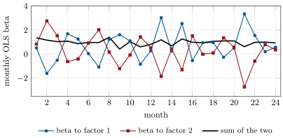
A factor model regresses a stock’s daily returns on five factors, month by month. Two of the factors move together, with correlation 0.97. Between the first month and the second, the stock’s beta to the first factor goes from 0.52 to $-1.59$ and its beta to the second from 0.84 to 2.76; their sum moves only from 1.36 to 1.17, and the second month’s fitted returns, recomputed with the first month’s betas, keep a correlation of 0.92 with its own fit. The regression is not wrong: it has been asked a question, how the exposure splits between two nearly identical factors, that three weeks of data cannot answer. This chapter is about least squares when its assumptions strain: the geometry that explains it, collinearity, the penalties that stabilise it, regressors measured with error, and the standard errors of regressions run on panels of stocks and months.

16.1 The geometry of least squares

Definition 16.1 (Ordinary least squares, hat matrix)

For $y \in \R^n$ and a full-rank design $X \in \R^{n \times k}$ , ordinary least squares (OLS) chooses $\hat\beta = (X^\top X)^{-1}X^\top y$ , the minimiser of $\lvert y - X\beta\rvert^2$ . The fitted values are $\hat y = Hy$ with the hat matrix $H = X(X^\top X)^{-1}X^\top$ , the orthogonal projection onto the column space of $X$ ; its diagonal entries $h_{ii}$ , which sum to $k$ , are the leverages of the observations.

The residual $y - \hat y = (I - H)y$ is orthogonal to every column of $X$ . An observation with leverage near one pulls the fit through itself: one bad print in a regressor is the worst kind of outlier, because it is far from the others in the direction the regression looks.

Theorem 16.2 (Gauss–Markov)

If $y = X\beta + \varepsilon$ with $\E[\varepsilon \mid X] = 0$ and $\Var(\varepsilon \mid X) = \sigma^2I$ , then $\hat\beta$ is unbiased with variance $\sigma^2(X^\top X)^{-1}$ , and every other linear unbiased estimator $Cy$ has variance larger by a positive semidefinite matrix.

Proof. Write $C = (X^\top X)^{-1}X^\top + D$ . Unbiasedness for every $\beta$ forces $DX = 0$ . Then $\Var(Cy) = \sigma^2CC^\top = \sigma^2(X^\top X)^{-1} + \sigma^2DD^\top$ , the cross terms vanishing because $DX = 0$ . ∎

The theorem is a statement about unbiased estimators; the rest of the chapter is about why a biased one is often better, and about what happens when $\Var(\varepsilon) \ne \sigma^2I$ or the regressor itself is noisy.

Theorem 16.3 (Frisch–Waugh–Lovell)

In the regression of $y$ on $(X_1, X_2)$ , the coefficient on $X_2$ equals the coefficient from regressing $M_1y$ on $M_1X_2$ , where $M_1 = I - X_1(X_1^\top X_1)^{-1}X_1^\top$ removes the part explained by $X_1$ ; the residuals of the two regressions coincide.

Proof. From $y = X_1\hat\beta_1 + X_2\hat\beta_2 + e$ with $e$ orthogonal to both blocks, apply $M_1$ : $M_1y = M_1X_2\hat\beta_2 + e$ , since $M_1X_1 = 0$ and $M_1e = e$ . As $e$ is orthogonal to $M_1X_2$ , this is the least-squares decomposition of $M_1y$ on $M_1X_2$ . ∎

A beta “controlling for” the market is the beta of the stock’s market-residual return on the factor’s market-residual return. The theorem is also the fastest way to see collinearity: the coefficient on $X_2$ is estimated from what is left of $X_2$ after $X_1$ , and when little is left, the estimate rests on little.

16.2 Collinearity

Definition 16.4 (Multicollinearity, variance inflation factor)

Multicollinearity is near-linear dependence among the columns of the design. The variance inflation factor of regressor $j$ is $\mathrm{VIF}_j = 1/(1 - R_j^2)$ , with $R_j^2$ the $R^2$ of regressing $x_j$ on the other regressors.

By the Frisch–Waugh–Lovell theorem, $\Var(\hat\beta_j) = \sigma^2/(n\,\widehat{\Var}(x_j)(1 - R_j^2))$ : the variance of a coefficient is the variance it would have alone, multiplied by its VIF. Two factors with correlation 0.97 have $\mathrm{VIF} = 1/(1 - 0.97^2) = 16.9$ (18.5 in the chapter’s sample), so each beta is four times noisier than it would be alone; the sum of the two betas, the exposure to their common direction, is not inflated at all.

Over 24 simulated months of 21 days, the stock’s true betas to the two collinear factors are 0.6 and 0.4. The monthly estimates have standard deviations of 1.21 and 1.23 across months, a sign opposite to the truth in 6 and 8 months, while their sum has a standard deviation of 0.23 (Figure 16.1); the betas to the three uncorrelated factors vary by 0.26 to 0.32. A risk report that lists the two betas separately reports noise; one that reports their sum, or projects the two factors on their first principal component, reports the exposure.

A stock’s betas to two factors with correlation 0.97, estimated each month from 21 daily returns (true values 0.6 and 0.4). The individual betas swing between -2.7 and 3.3; their sum stays near its true value of 1.0 (standard deviation 0.23). Data: the chapter’s tutorial, seeded. — **Figure 16.1.** A stock’s betas to two factors with correlation 0.97, estimated each month from 21 daily returns (true values 0.6 and 0.4). The individual betas swing between $-2.7$ and $3.3$ ; their sum stays near its true value of 1.0 (standard deviation 0.23). Data: the chapter’s tutorial, seeded.

16.3 Ridge, lasso and elastic net

Definition 16.5 (Regularisation, ridge, lasso, elastic net)

Regularisation adds a penalty on the size of the coefficients to the least-squares objective. Ridge regression minimises $\lvert y - X\beta\rvert^2 + \lambda\lvert\beta\rvert_2^2$ ; the lasso minimises $\frac1{2n}\lvert y - X\beta\rvert^2 + \lambda\lvert\beta\rvert_1$ ; the elastic net uses the penalty $\lambda\bigl(\alpha\lvert\beta\rvert_1 + \frac{1 - \alpha}2\lvert\beta\rvert_2^2\bigr)$ , $\alpha \in [0, 1]$ .

Proposition 16.6 (Ridge shrinks along the singular directions)

If $X = UDV^\top$ is a thin singular value decomposition, the ridge estimate is $\hat\beta_\lambda = \sum_jv_j\frac{d_j}{d_j^2 + \lambda}u_j^\top y$ : the least-squares coefficient along each right singular vector $v_j$ is multiplied by $d_j^2/(d_j^2 + \lambda)$ .

Proof. $\hat\beta_\lambda = (X^\top X + \lambda I)^{-1}X^\top y = V(D^2 + \lambda I)^{-1}DU^\top y$ , and least squares is the case $\lambda = 0$ , with factor $1/d_j$ along $v_j$ . ∎

Collinear directions have small singular values, and they are the ones ridge shrinks: for the two factors above, the difference $F_1 - F_2$ has a small singular value and its coefficient is pulled toward zero, while the sum is left almost alone. Ridge is the posterior mean under a normal prior on $\beta$ (chapter 14). The lasso’s absolute-value penalty has a corner at zero: for an orthonormal design its solution is the least-squares coefficient soft-thresholded, $\operatorname{sign}(b)\max(|b| - \lambda, 0)$ , so it sets small coefficients exactly to zero and selects variables. Within a block of correlated predictors it tends to pick one and drop the others, somewhat arbitrarily; the elastic net’s ridge part spreads the weight across the block. The lasso and elastic net are computed by cyclic coordinate descent, each coordinate being a one-dimensional soft-thresholding (Friedman, Hastie and Tibshirani, 2010).

Definition 16.7 (Cross-validation)

Cross-validation chooses a penalty by fitting on part of the data and measuring the prediction error on the rest, over several splits. With time series, every training set must precede its test set, with a gap (a purge) at least as long as the dependence between the targets, so that no information from the test period leaks into the fit.

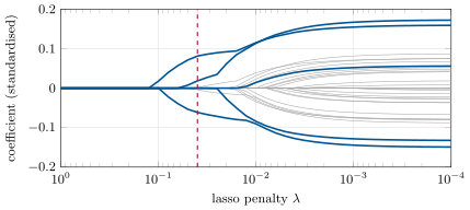
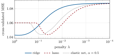
The tutorial predicts a daily return from thirty predictors in three blocks of ten, correlated 0.8 within each block; five predictors carry signal, and the signal is weak (a perfect model would explain 5.0% of the variance out of sample). The first 1 500 days are split into five expanding folds with a purge of five days, and the last 500 are the test. OLS on all thirty predictors explains 1.5% of the test variance; ridge at the cross-validated penalty 3.5%, the lasso 3.4%, the elastic net 3.2%. The lasso keeps five predictors, three of them right; in the two blocks where it errs it has kept a correlated neighbour of a true predictor (Figures 16.2 and 16.3).

Lasso path of the thirty standardised predictors as the penalty falls from 1 to 10-4: the five true signals in blue, the twenty-five noise predictors in grey, and the cross-validated penalty 0.040 (dashed), where five coefficients are nonzero. Data: the chapter’s tutorial, seeded. — **Figure 16.2.** Lasso path of the thirty standardised predictors as the penalty falls from 1 to $10^{-4}$ : the five true signals in blue, the twenty-five noise predictors in grey, and the cross-validated penalty 0.040 (dashed), where five coefficients are nonzero. Data: the chapter’s tutorial, seeded.

**Figure 16.3.** Time-ordered cross-validation error of the three penalised regressions against the penalty (five expanding folds with a five-day purge, on the first 1 500 days). Each curve has an interior minimum: too little penalty fits noise, too much discards signal. Data: the chapter’s tutorial, seeded.

16.4 Weighted and errors-in-variables regression

Definition 16.8 (Weighted and generalised least squares)

Weighted least squares minimises $\sum_iw_i(y_i - x_i^\top\beta)^2$ , with weights inversely proportional to the variance of each observation’s error. Generalised least squares minimises $(y - X\beta)^\top\Omega^{-1}(y - X\beta)$ for an error covariance $\Omega$ ; it is OLS after multiplying the model by $\Omega^{-1/2}$ , and it is the efficient linear unbiased estimator when $\Omega$ is known.

When $\Omega$ is unknown, the usual choice in finance is OLS with a standard error that does not assume it away: the sandwich of chapter 11, HAC for time series, clustered for panels (below).

Definition 16.9 (Errors-in-variables, attenuation bias, total least squares)

An errors-in-variables model observes the regressor with noise, $\tilde x = x + u$ , with $u$ independent of $x$ and of the equation error. The resulting shrinkage of the OLS slope toward zero is the attenuation bias. Total least squares fits the line minimising the sum of squared perpendicular distances, which is consistent when the errors in $x$ and in $y$ have equal variances.

Proposition 16.10 (The attenuation factor)

If $y = \beta x + \varepsilon$ and $\tilde x = x + u$ with $x$ , $u$ , $\varepsilon$ independent, the OLS slope of $y$ on $\tilde x$ converges to $\lambda\beta$ with $\lambda = \Var(x)/(\Var(x) + \Var(u))$ .

Proof. $\Cov(y, \tilde x) = \beta\Var(x)$ and $\Var(\tilde x) = \Var(x) + \Var(u)$ ; the slope is their ratio. ∎

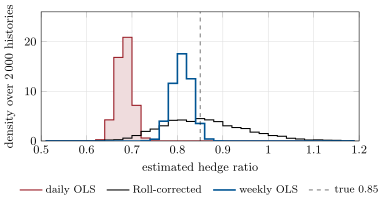
A desk hedges a bond with a bond future, and estimates the hedge ratio by regressing the bond’s daily price changes on the future’s. The bond is marked at a synchronous mid at the close; the future’s recorded daily price is its last trade before the close, stale by a few minutes and at bid or ask. Model the recorded level as the true level plus an independent error of standard deviation 0.14 points; the future’s true daily change has standard deviation 0.40, and the bond moves 0.85 times the future plus an idiosyncratic 0.05. The recorded change carries the difference of two level errors, of variance $2 \times 0.14^2 = 0.039$ , so $\lambda = 0.16/(0.16 + 0.039) = 0.80$ . On two years of seeded data the OLS hedge ratio is 0.68, and across 2 000 simulated histories it averages 0.683 with a standard deviation of 0.017: precisely wrong.

Two corrections come from the structure of the error. A level error makes consecutive recorded changes negatively correlated, with first autocovariance $-\sigma_e^2$ (Roll’s 1984 argument for the bid-ask spread), so $\hat\lambda = (\hat\gamma(0) + 2\hat\gamma(1))/\hat\gamma(0)$ estimates the attenuation from the future’s own series; here the first autocorrelation is $-0.098$ , $\hat\lambda = 0.80$ , and the corrected ratio is 0.85. Across histories this correction is unbiased (0.862 on average) but noisy (standard deviation 0.095). Alternatively, weekly changes add five days of true movement to the same two level errors, so their attenuation is only $5 \times 0.16/(5 \times 0.16 + 0.039) = 0.95$ : the weekly regression gives 0.80 on this history, 0.810 on average with a standard deviation of 0.022 (Figure 16.4). Total least squares gives 0.74: its assumption of equal error variances is false here.

**Figure 16.4.** Sampling distributions of three hedge-ratio estimates over 2 000 simulated two-year histories: daily OLS on the noisy future prices (mean 0.683, attenuated by 0.80), the same divided by the attenuation estimated from the future’s first autocorrelation (mean 0.862, standard deviation 0.095), and OLS on weekly changes (mean 0.810, standard deviation 0.022). Data: the chapter’s tutorial, seeded.

The cost is in the residual. Measured against the true synchronous changes, the hedge at the true ratio leaves a daily residual of 0.049 points; at the daily OLS ratio 0.086, 74% more; at the corrected ratio 0.049; at the weekly ratio 0.053. Unhedged, the bond moves 0.34 a day.

16.5 Cross-sectional regressions over time, and panels

Definition 16.11 (Panel data, fixed effects)

Panel data observe many units (stocks, funds, counterparties) over many periods. A fixed effects regression gives each unit (or period) its own intercept, which by the Frisch–Waugh–Lovell theorem is the same as demeaning every variable within the unit.

Definition 16.12 (Fama–MacBeth regression, clustered standard errors)

A Fama–MacBeth regression (Fama and MacBeth, 1973) runs one cross-sectional regression per period and reports the time-series mean of the slopes, with standard error their standard deviation over $\sqrt T$ . Clustered standard errors compute the sandwich variance with the scores summed within clusters (firms, or periods), allowing any correlation inside a cluster and none across clusters.

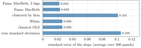
The Fama–MacBeth standard error is right when the slopes are independent over time; a period effect (all stocks’ residuals moving together in a month) is handled, since each month’s slope absorbs it. A persistent firm effect is not: if both a characteristic and the residual have a component fixed for each firm, every month’s slope shares the same error, which the time-series standard deviation cannot see and a Newey–West correction with a few lags cannot see either (Petersen, 2009). In a simulated panel of 100 firms over 60 months with firm effects making up half the variance of the characteristic and of the residual, the slope’s true standard deviation across 500 panels is 0.105. Classical and White standard errors average 0.026, the Fama–MacBeth one 0.023 (0.022 with three Newey–West lags), and only the standard error clustered by firm, 0.101, is right (Figure 16.5).

**Figure 16.5.** Standard errors of a panel slope when the characteristic and the residual both have a persistent firm component: only clustering by firm recovers the true sampling standard deviation (0.105); the classical, White and Fama–MacBeth standard errors understate it about fourfold. Data: the chapter’s tutorial, seeded.

16.6 Tutorial: the hedge ratio that shrank

Goal. Stabilise a collinear regression, select predictors with time-ordered cross-validation, and repair an attenuated hedge ratio. End state: Figures 16.2, 16.3 and 16.4, the test $R^2$ of 1.5% (OLS) and 3.5% (ridge), and the hedge ratios 0.68, 0.85 and 0.80.

Ridge through the SVD and the elastic net by coordinate descent.

def ridge(X, y, lam: float) -> np.ndarray:
    """Each singular direction's least-squares coefficient multiplied by d^2 / (d^2 + lam)."""
    u, d, vt = np.linalg.svd(np.asarray(X, dtype=float), full_matrices=False)
    return vt.T @ ((d / (d * d + lam)) * (u.T @ np.asarray(y, dtype=float)))


def elastic_net(X, y, lam: float, alpha: float = 1.0, beta0=None, tol: float = 1e-9,
                max_iter: int = 10_000) -> np.ndarray:
    """Cyclic coordinate descent with soft thresholding (alpha = 1: lasso; alpha = 0: ridge)."""
    X, y = np.asarray(X, dtype=float), np.asarray(y, dtype=float)
    n, k = X.shape
    b = np.zeros(k) if beta0 is None else np.array(beta0, dtype=float)
    col_sq = np.sum(X * X, axis=0) / n
    r = y - X @ b
    for _ in range(max_iter):
        delta = 0.0
        for j in range(k):
            if col_sq[j] == 0:
                continue
            old = b[j]
            rho = X[:, j] @ r / n + col_sq[j] * old
            new = math.copysign(max(abs(rho) - lam * alpha, 0.0), rho) / (col_sq[j] + lam * (1 - alpha))
            if new != old:
                r -= X[:, j] * (new - old)
                b[j] = new
                delta = max(delta, abs(new - old))
        if delta < tol:
            break
    return b

Listing 16.1. Ridge and elastic net. code/firm/linreg/firm_linreg.py

Time-ordered folds with a purge.

def time_series_folds(n: int, n_folds: int, purge: int = 0, min_train: int | None = None) -> list:
    """Expanding-window folds: the data are cut into n_folds + 1 blocks; fold f trains on blocks 0..f
    (minus the last `purge` observations) and tests on block f + 1."""
    edges = np.linspace(0, n, n_folds + 2).astype(int)
    folds = []
    for f in range(n_folds):
        train_end = edges[f + 1] - purge
        if min_train is not None and train_end < min_train:
            continue
        folds.append((np.arange(0, max(train_end, 0)), np.arange(edges[f + 1], edges[f + 2])))
    return folds

Listing 16.2. Expanding-window cross-validation folds. code/firm/linreg/firm_linreg.py

Run fit_all(), hedge(), hedge_mc() and panel_truth() in qm_linreg.py, then fig_linreg.py.

What to change next. Replace the two collinear factors by their sum and difference and watch the difference’s beta alone carry the noise; shorten the purge to zero with overlapping five-day targets and measure how much cross-validation flatters the fit.

16.7 Build: the regression module

Purpose. Every regression the miniature firm runs (betas, hedge ratios, signal fits, panel tests) goes through one module whose standard errors are chosen, not defaulted.

Interface. ols(X, y, cov, lags, groups) with cov in classical, hc, hac, cluster; vif(X); ridge(X, y, lam); elastic_net(X, y, lam, alpha); time_series_folds(n, n_folds, purge); fama_macbeth(ys, Xs, lags); tls(x, y).

Rules. The covariance type is a required choice in reports; predictors are standardised on the training fold only; folds never train on data after their test block; warm starts along a penalty path.

Acceptance tests. code/firm/linreg/tests/: White standard errors match the simulated sampling spread under heteroskedasticity; the Frisch–Waugh–Lovell identity; the VIF of two variables with correlation 0.97; ridge equals its normal equations and the elastic net with $\alpha = 0$ equals ridge; the lasso soft-thresholds an orthonormal design; purged folds; Fama–MacBeth on independent periods.

Stretch. Deming regression with a known error-variance ratio; the adaptive lasso; two-way clustering by firm and month.

Sources and further reading

R. Frisch and F. V. Waugh, “Partial time regressions as compared with individual trends”, Econometrica 1, 1933; M. C. Lovell, Journal of the American Statistical Association 58, 1963.
A. E. Hoerl and R. W. Kennard, “Ridge regression: biased estimation for nonorthogonal problems”, Technometrics 12, 1970.
R. Tibshirani, “Regression shrinkage and selection via the lasso”, Journal of the Royal Statistical Society B 58, 1996.
H. Zou and T. Hastie, “Regularization and variable selection via the elastic net”, Journal of the Royal Statistical Society B 67, 2005.
J. Friedman, T. Hastie and R. Tibshirani, “Regularization paths for generalized linear models via coordinate descent”, Journal of Statistical Software 33, 2010.
E. F. Fama and J. D. MacBeth, “Risk, return, and equilibrium: empirical tests”, Journal of Political Economy 81, 1973.
M. A. Petersen, “Estimating standard errors in finance panel data sets: comparing approaches”, Review of Financial Studies 22, 2009.
R. Roll, “A simple implicit measure of the effective bid-ask spread in an efficient market”, Journal of Finance 39, 1984.

16.8 Exercises

Exercise 16.1 ★

Two regressors have correlation 0.9. What is the variance inflation factor, and by what factor does each coefficient’s standard error grow?

Solution

Solution of Exercise 16.1.

$R_j^2 = 0.81$ , so $\mathrm{VIF} = 1/0.19 = 5.3$ and each standard error grows by $\sqrt{5.3} = 2.3$ .

Exercise 16.2 ★

A regressor’s true variance is 1 and it is measured with independent noise of variance 0.25. If the true slope is 2, what does OLS estimate?

Solution

Solution of Exercise 16.2.

$\lambda = 1/(1 + 0.25) = 0.8$ , so OLS estimates $0.8 \times 2 = 1.6$ .

Exercise 16.3 ★

Show that the leverages $h_{ii}$ sum to $k$ , the number of columns of $X$ .

Solution

Solution of Exercise 16.3.

$\sum_ih_{ii} = \operatorname{tr}H = \operatorname{tr}\bigl(X(X^\top X)^{-1}X^\top\bigr) = \operatorname{tr}\bigl((X^\top X)^{-1}X^\top X\bigr) = \operatorname{tr}I_k = k$ .

Exercise 16.4 ★★

For an orthonormal design ( $X^\top X = nI$ ), derive the lasso solution coordinate by coordinate.

Solution

Solution of Exercise 16.4.

With $X^\top X = nI$ the objective separates: $\frac1{2n}\lvert y - X\beta\rvert^2 = \mathrm{const} + \frac12\sum_j(\beta_j - b_j)^2$ with $b = X^\top y/n$ the least-squares coefficient. Each coordinate minimises $\frac12(\beta_j - b_j)^2 + \lambda|\beta_j|$ , whose solution is $\operatorname{sign}(b_j)\max(|b_j| - \lambda, 0)$ : soft thresholding.

Exercise 16.5 ★★

A future’s recorded daily changes have variance 0.199 and first autocovariance $-0.0196$ . Estimate the level-error variance and the attenuation factor of a daily hedge regression, and the attenuation of a weekly one.

Solution

Solution of Exercise 16.5.

The level-error variance is $-\gamma(1) = 0.0196$ (standard deviation 0.14), so $\hat\lambda = (0.199 - 2 \times 0.0196)/0.199 = 0.80$ . Weekly, the true variance is $5 \times (0.199 - 0.0392) = 0.80$ against the same $0.0392$ of error: $\lambda_5 = 0.80/0.839 = 0.95$ .

Exercise 16.6 ★★

With the two collinear factors of the chapter ( $\rho = 0.97$ , unit variances), which linear combination of the two betas does the data pin down, and how much more precisely than each beta?

Solution

Solution of Exercise 16.6.

With $X^\top X \approx n\left(\begin{smallmatrix}1 & \rho\\ \rho & 1\end{smallmatrix}\right)$ , $\Var(\hat\beta_1) = \sigma^2/(n(1 - \rho^2)) = 16.9\sigma^2/n$ while $\Var(\hat\beta_1 + \hat\beta_2) = 2\sigma^2/(n(1 + \rho)) = 1.02\sigma^2/n$ . The sum, the exposure to the common direction, is pinned down about four times more precisely (in standard deviation) than either beta; the difference, with variance $2\sigma^2/(n(1 - \rho)) = 66.7\sigma^2/n$ , is where the noise lives.

Exercise 16.7 ★★★

Coding. Simulate the chapter’s panel with firm effects and compare the average classical, clustered and Fama–MacBeth standard errors with the true sampling standard deviation of the slope over 500 panels.

Solution

Solution of Exercise 16.7.

panel_truth(): true standard deviation 0.105; classical 0.026 and White 0.026; clustered by firm 0.101; Fama–MacBeth 0.023 (0.022 with three Newey–West lags). The firm effect is common to every month’s slope, so neither the classical formula nor the time-series spread of the monthly slopes sees it; clustering by firm does.

Exercise 16.8 ★★★

Find the flaw. “We chose the lasso penalty by ten-fold cross-validation with random folds on five years of daily data, predicting each stock’s next twenty-day return; the cross-validated $R^2$ is 8%.”

Solution

Solution of Exercise 16.8.

Random folds put days from the future into the training set of every test day, and with twenty-day targets overlapping by nineteen days, neighbouring observations share most of their target: the model is tested on returns it has effectively seen. Use expanding (or rolling) folds in time order with a purge of at least twenty days between training and test, and expect a far lower $R^2$ ; also count the penalties and specifications tried (chapter 12).

16.9 Problem: The Hedge Ratio That Shrank

Problem 16.1

Weekend problem — hedging a bond with a future whose prices are noisy

A bond’s daily price change is 0.85 times the future’s true change plus an idiosyncratic 0.05 points; the future’s true change has standard deviation 0.40 points; its recorded daily price carries an independent level error of standard deviation 0.14. Two years (500 days) of the chapter’s seeded data are available.

Part I — The naive hedge.

What hedge ratio does daily OLS give?
What attenuation factor does the model predict, and what does it imply for the average OLS ratio?
Across 2 000 simulated histories, what are the mean and standard deviation of the daily OLS ratio?
Why is a precise estimate not a correct one here?
What residual daily risk does the OLS ratio leave, against the true ratio’s?

Part II — Corrections.

What is the first autocorrelation of the recorded future changes, and what does it imply for $\hat\lambda$ ?
What is the corrected ratio, and its residual risk?
What attenuation does a weekly regression suffer, and what ratio does it give?
What are the mean and standard deviation of the corrected and weekly ratios across histories?
What does total least squares give, and why is it wrong here?

Part III — Beyond the hedge.

What would the attenuation be with a level error of 0.07 instead of 0.14?
How would synchronous prices (both marked at the same instant, at mid) change the problem?
If the hedge ratio were estimated on monthly changes, what would be gained and lost?
Could the collinearity of the chapter’s factor model be repaired by the same means?
How would you check the estimated ratio before trading it?

Part IV — Judgement.

Which ratio would you use, and why?
What should the data team change?
When is the attenuation of a regression slope harmless?
State the named result: the attenuation factor, the corrected ratio, and the residual risk each leaves.
In one sentence: what does noise in a regressor do that noise in the dependent variable does not?

Solution

Solution of Problem 16.1.

1. 0.68. 2. $\lambda = 0.16/(0.16 + 2 \times 0.14^2) = 0.80$ , so on average $0.80 \times 0.85 = 0.683$ . 3. Mean 0.683, standard deviation 0.017. 4. The noise in the regressor biases the slope; more data shrink the variance around the wrong value, not the bias. 5. 0.086 points a day against 0.049 at the true ratio, 74% more. 6. $-0.098$ ; $\hat\lambda = 1 + 2 \times (-0.098) = 0.80$ . 7. $0.68/0.80 = 0.85$ , residual 0.049. 8. $\lambda_5 = 0.95$ ; the weekly ratio is 0.80, residual 0.053. 9. Corrected: mean 0.862, standard deviation 0.095. Weekly: mean 0.810, standard deviation 0.022. 10. 0.74; it assumes the error variances in the bond and the future are equal, while here the future’s is 0.039 and the bond’s residual 0.0025. 11. $0.16/(0.16 + 2 \times 0.07^2) = 0.94$ . 12. It removes the problem: no level error, no attenuation, and the daily OLS ratio is unbiased. 13. Monthly, $\lambda_{21} = 21 \times 0.16/(21 \times 0.16 + 0.039) = 0.99$ , almost no bias, but only 24 observations in two years, so a noisy ratio; the weekly regression is the compromise. 14. No: collinearity is a lack of independent variation, not noise in a regressor. Aggregating does not separate the factors; only reporting their sum, penalising, or finding data where they move apart does. 15. Compare with the duration-based ratio, test the hedged P&L out of sample, and check the ratio’s stability across periods and horizons. 16. The corrected or duration-based ratio near 0.85, cross-checked by the weekly 0.80; not the daily OLS 0.68. 17. Record synchronous mids for the future at the bond’s marking time. 18. When the goal is prediction from the noisy regressor itself (the attenuated slope is then the best linear predictor), rather than the structural relation. 19. Named result: the hedge ratio that shrank: stale, bid-ask-noisy future prices attenuate the daily OLS hedge ratio by 0.80, from 0.85 to 0.68; the ratio corrected from the future’s own first autocorrelation is 0.85; the residual risk is 0.086 points a day at 0.68 against 0.049 at 0.85 (0.053 at the weekly 0.80). 20. It biases the slope toward zero, while noise in the dependent variable only adds variance.

16.10 Interview questions

Interview question 16.1 ★ researcher, mle

Two of your regressors have correlation 0.97. What happens to their coefficients, and what do you do?

Solution

Solution of Interview question 16.1.

Each coefficient’s variance is inflated by $1/(1 - 0.97^2) = 17$ ; the individual coefficients swing and can flip sign, while their sum is well determined. Report the sum or the principal-component exposure, penalise (ridge), or drop one factor.

What the interviewer is looking for: The VIF, the stable combination, and a remedy chosen for the question asked.

Interview question 16.2 ★★ researcher, trader

Your regression hedge ratio is 0.68 but the duration ratio says 0.85. What could explain the gap?

Solution

Solution of Interview question 16.2.

Attenuation from noise in the regressor: asynchronous or stale prices, bid-ask bounce in the future’s prints. Also a changing relation (the sample spans different regimes), or the wrong horizon. Check the future’s first autocorrelation, rerun on weekly changes, and use synchronous prices.

What the interviewer is looking for: Errors-in-variables as the first suspect, with a diagnostic and a fix.

Interview question 16.3 ★★ mle, researcher

Ridge or lasso: what does each do to correlated predictors?

Solution

Solution of Interview question 16.3.

Ridge shrinks along the small singular directions and spreads weight across a correlated block; the lasso sets coefficients to zero and tends to keep one member of a block, somewhat arbitrarily; the elastic net keeps groups together while still selecting.

What the interviewer is looking for: Shrinkage versus selection, and the behaviour within correlated groups.

Interview question 16.4 ★★ mle, researcher

How do you cross-validate a model that predicts twenty-day returns from daily data?

Solution

Solution of Interview question 16.4.

Folds in time order, training before testing, with a purge gap of at least the target’s horizon (twenty days) so overlapping targets do not leak, and possibly an embargo after the test block; standardise and choose features inside each training fold only.

What the interviewer is looking for: Time order, purge for overlap, and no preprocessing on the full sample.

Interview question 16.5 ★★ researcher

When are Fama–MacBeth standard errors wrong, and what do you use instead?

Solution

Solution of Interview question 16.5.

When the regressors and residuals have persistent firm effects: every period’s slope shares the same error, so the time-series standard deviation understates the uncertainty. Use standard errors clustered by firm (or by firm and period when both effects exist).

What the interviewer is looking for: Which dependence each method handles: Fama–MacBeth handles time effects, clustering by firm handles firm effects.

Interview question 16.6 ★★★ researcher, mle

State and prove the Frisch–Waugh–Lovell theorem, and give a use of it on a trading desk.

Solution

Solution of Interview question 16.6.

The coefficient on $X_2$ in the regression on $(X_1, X_2)$ equals the slope of $M_1y$ on $M_1X_2$ , the parts orthogonal to $X_1$ ; proof by applying $M_1$ to the normal equations. On a desk: a stock’s beta to a sector after removing the market is the slope of market-residual returns; a signal’s marginal value after existing signals is its fit on residualised returns.

What the interviewer is looking for: The projection argument and a concrete residualisation.

Terms defined in this chapter

See all 2333 terms in the glossary