17Linear Time Series

The spread between the ten-year and the two-year Treasury yields, the 2s10s that a steepener trades, has a daily autocorrelation of 0.9987 over fifty years. A regression of tomorrow’s spread on today’s gives a slope of 0.99875 with a standard error of 0.00045: a $t$-statistic of $-2.79$ against a slope of one, a one-sided $p$-value of 0.003 by the normal table. The spread seems to mean-revert, with a half-life of 552 trading days. But if the spread had a unit root, the normal table would be the wrong one: the right one puts the 5% critical value at $-2.86$, and the evidence falls short. This chapter is about the models that describe such series and the tests that tell them apart: stationarity and the autocorrelation function, autoregressive and moving-average models, the spectral view, unit roots and the regressions they make spurious, and long memory.

17.1 Stationarity and autocorrelation

Definition 17.1 (Stationary process, weak stationarity, white noise)

A process $(X_t)$ is a stationary process (strictly) if the joint law of $(X_{t_1 + h}, \dots, X_{t_k + h})$ does not depend on $h$. It has weak stationarity if its mean is constant and $\Cov(X_t, X_{t+h})$ depends only on $h$. White noise is a weakly stationary sequence with mean zero and no autocorrelation at any nonzero lag.

Definition 17.2 (Autocovariance, autocorrelation and partial autocorrelation functions)

For a weakly stationary process, the autocovariance function is $\gamma(h) = \Cov(X_t, X_{t+h})$, and the autocorrelation function is $\rho(h) = \gamma(h)/\gamma(0)$. The partial autocorrelation function at lag $h$ is the last coefficient $\phi_{hh}$ of the best linear predictor of $X_{t+h}$ from $X_{t+h-1}, \dots, X_t$: the correlation at lag $h$ once the intermediate lags are accounted for.

Under white noise the sample autocorrelations are approximately independent $\mathcal N(0, 1/n)$, whence the $\pm 2/\sqrt n$ bands of every correlogram. The decomposition that justifies the models of the next section is Wold’s (1938): every weakly stationary, purely nondeterministic process is an infinite moving average $X_t = \mu + \sum_{j \ge 0}\psi_j\varepsilon_{t-j}$ of its one-step prediction errors $\varepsilon_t$, a white noise, with $\psi_0 = 1$ and $\sum_j\psi_j^2 < \infty$.

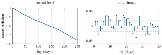
The 2s10s spread’s correlogram (Figure 17.1) is the signature of a nearly nonstationary level: autocorrelations that start at 0.9987 and fall almost linearly over a year of lags. Its daily changes are nearly white noise, with a standard deviation of 4.6 basis points and autocorrelations of 0.015, 0.015 and $-0.027$ at the first three lags, within the band $\pm 0.018$ for the first two.

17.2 Autoregressive and moving-average models

Definition 17.3 (Autoregressive, moving-average and ARMA processes)

With $(\varepsilon_t)$ white noise of variance $\sigma^2$: an autoregressive process of order $p$, AR($p$), satisfies $X_t = c + \sum_{i=1}^p\phi_iX_{t-i} + \varepsilon_t$; a moving-average process of order $q$, MA($q$), is $X_t = \mu + \varepsilon_t + \sum_{j=1}^q\vartheta_j\varepsilon_{t-j}$; an ARMA process combines them, $\phi(L)X_t = c + \vartheta(L)\varepsilon_t$ with $\phi(z) = 1 - \sum_i\phi_iz^i$, $\vartheta(z) = 1 + \sum_j\vartheta_jz^j$ and $L$ the lag operator.

Proposition 17.4 (Stationarity and invertibility of ARMA)

The ARMA equation has a unique weakly stationary causal solution $X_t = \mu + \sum_{j \ge 0}\psi_j\varepsilon_{t-j}$ if and only if every root of $\phi(z)$ lies outside the unit circle; it is invertible, $\varepsilon_t = \sum_{j \ge 0}\pi_jX_{t-j}$ up to a constant, if and only if every root of $\vartheta(z)$ does, the polynomials having no common root.

For the AR(1) $X_t = c + \phi X_{t-1} + \varepsilon_t$, the condition is $|\phi| < 1$, the autocorrelations are $\phi^h$, and a deviation from the mean decays by half in $\ln(1/2)/\ln\phi$ periods, the half-life of chapter 4’s Ornstein–Uhlenbeck process sampled daily. An AR($p$) has a partial autocorrelation function that cuts off after lag $p$; an MA($q$) has an autocorrelation function that cuts off after lag $q$. The orders are chosen by an information criterion.

Definition 17.5 (Information criterion)

An information criterion ranks models by fit penalised for size: Akaike’s $\mathrm{AIC} = -2\ell + 2k$ and Schwarz’s $\mathrm{BIC} = -2\ell + k\ln n$, for maximised log-likelihood $\ell$ and $k$ parameters; the smallest wins.

AIC aims at prediction and tends to choose large models; BIC is consistent for the true order when there is one. On the 2s10s daily changes AIC chooses an AR(10) whose coefficients are all below 0.035 in absolute value: statistically detectable with 12 574 days, economically nothing.

17.3 The spectral view

Definition 17.6 (Spectral density, periodogram)

The spectral density of a weakly stationary process with summable autocovariances is $f(\omega) = \frac1{2\pi}\sum_h\gamma(h)e^{-ih\omega}$, $\omega \in [-\pi, \pi]$: the decomposition of its variance by frequency, $\gamma(0) = \int_{-\pi}^\pi f$. The periodogram $I(\omega_j) = \frac1{2\pi n}\bigl\lvert\sum_tX_te^{-it\omega_j}\bigr\rvert^2$ at the Fourier frequencies $\omega_j = 2\pi j/n$ is its sample counterpart.

White noise has a flat spectrum, $\sigma^2/2\pi$; an AR(1) with $\phi$ near one concentrates its variance at low frequencies, $f(\omega) = \sigma^2/(2\pi|1 - \phi e^{-i\omega}|^2)$. The periodogram is asymptotically unbiased but not consistent: each ordinate is approximately $f(\omega_j)$ times an exponential variable, however long the sample, so it must be smoothed or averaged. Its low-frequency end is where persistence shows, and it is the basis of the long-memory estimate of the last section. $f(0) = \frac1{2\pi}\sum_h\gamma(h)$ is, up to $2\pi$, the long-run variance of chapter 11.

17.4 Unit roots

Definition 17.7 (Unit root, spurious regression)

A process has a unit root if its autoregressive polynomial has a root at $z = 1$: its first difference is stationary but the level is not, like a random walk. A spurious regression is a regression between independent processes with unit roots whose usual $t$-statistics and $R^2$ indicate a relation that does not exist.

Granger and Newbold (1974) showed the problem by simulation, and it is easy to repeat: regressing one random walk of 500 steps on another, independent one, the slope’s $t$-statistic exceeds 1.96 in absolute value in 89% of 5 000 trials, with a median $R^2$ of 0.17. The residual inherits the unit root, the observations are not independent, and every formula that assumed they were is wrong. The same failure hits the test of $\phi = 1$ itself.

Definition 17.8 (Dickey–Fuller test)

The Dickey–Fuller test of a unit root regresses $\Delta X_t$ on $X_{t-1}$ (with a constant, and a trend if wanted) and compares the $t$-statistic $\tau$ of the coefficient on $X_{t-1}$ with the Dickey–Fuller distribution rather than the normal; the augmented version adds lagged differences $\Delta X_{t-k}$ to absorb short-run dependence (Said and Dickey, 1984).

Under the unit root and with a constant, $\tau$ converges to $\bigl(\frac12(W(1)^2 - 1) - W(1)\int_0^1W\bigr)/\bigl(\int_0^1W^2 - (\int_0^1W)^2\bigr)^{1/2}$ for a standard Brownian motion $W$, a functional that is neither normal nor centred at zero (Figure 17.2). Its quantiles have no closed form; MacKinnon’s (2010) response surfaces give the 1%, 5% and 10% critical values $-3.43$, $-2.86$ and $-2.57$ for large samples. The chapter’s own simulation of 20 000 random walks of 500 steps gives $-3.46$, $-2.89$ and $-2.57$, against MacKinnon’s $-3.44$, $-2.87$ and $-2.57$ at that length.

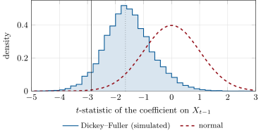
For the 2s10s spread, $\tau = -2.79$ with no lagged differences: not significant at 5%, significant at 10%. The augmented test depends on the lags: $-2.74$ with five, $-3.13$ with ten, $-3.55$ with twenty; AIC, searching up to forty, chooses 34 and $-3.14$. On the sample since 1990 the Dickey–Fuller statistic is $-2.01$. The honest reading is that the data cannot decide: the spread mean-reverts too slowly for fifty years of daily data to tell it from a random walk.

Proposition 17.9 (Kendall’s bias of the AR(1) coefficient)

For a stationary AR(1) with an estimated mean, the least-squares coefficient satisfies $\E[\hat\phi] - \phi = -(1 + 3\phi)/n + O(n^{-2})$ (Kendall, 1954).

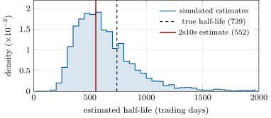
The bias is small in the coefficient and large in the half-life, because the half-life divides by $\ln\phi$, close to zero. The spread’s estimate 0.99875, corrected by $(1 + 3 \times 0.99875)/12\,574 = 0.00032$, becomes 0.99906, and the half-life grows from 552 trading days (2.2 years) to 739 (2.9 years). The correction is an average: simulating 4 000 histories of 12 574 days from an AR(1) with $\phi = 0.99906$, the estimated half-life has median 576 days and a 10–90% range of 352 to 969 days (Figure 17.3), and in 57% of the histories the Dickey–Fuller test does not reject the unit root at 5%, although there is none.

17.5 Long memory

Definition 17.10 (Long memory, fractional differencing, Hurst exponent)

A stationary process has long memory if its autocorrelations decay like a power, $\rho(h) \sim ch^{2d-1}$ with $0 < d < \frac12$, so that they are not summable. Fractional differencing applies $(1 - L)^d = \sum_{j \ge 0}w_jL^j$ with $w_0 = 1$, $w_j = w_{j-1}(j - 1 - d)/j$; the ARFIMA$(0, d, 0)$ process is $(1 - L)^dX_t = \varepsilon_t$ (Granger and Joyeux, 1980; Hosking, 1981). The Hurst exponent is $H = d + \frac12$, measured by the growth of ranges or variances of partial sums like $n^H$ (Hurst, 1951).

Definition 17.11 (Fractional Brownian motion)

Fractional Brownian motion with Hurst exponent $H \in (0, 1)$ is the centred Gaussian process with $B_H(0) = 0$ and $\E[B_H(t)B_H(s)] = \frac12(t^{2H} + s^{2H} - |t - s|^{2H})$ (Mandelbrot and Van Ness, 1968). For $H = \frac12$ it is Brownian motion; for $H > \frac12$ its increments are positively correlated with power-law decay, for $H < \frac12$ negatively.

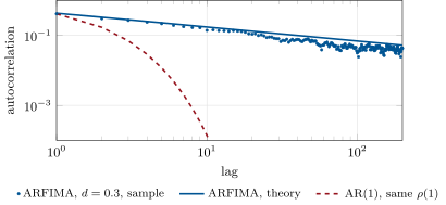
For $H \ne \frac12$ fractional Brownian motion is not a semimartingale, so the Itô calculus of chapter 3 does not apply to it, and a price that followed it would admit arbitrage; it is a model for volatility and for slowly mean-reverting quantities, not for prices. The difference between long and short memory is in the tail of the correlogram (Figure 17.4): an ARFIMA with $d = 0.3$ and an AR(1) with the same first autocorrelation, 0.41, differ by a factor of a thousand at lag 10. On 20 000 simulated observations the rescaled-range estimate of $H$ is 0.78 and the log-periodogram (Geweke–Porter-Hudak) estimate 0.71, for a true 0.8; on white noise they give 0.53 and 0.46, the rescaled range being biased upward in short blocks.

The spread’s daily changes give a log-periodogram estimate $H = 0.34$ from the lowest $\sqrt n = 112$ frequencies, that is $d = -0.16$ with a standard error of $\pi/\sqrt{24 \times 112} = 0.06$: the changes are over-differenced, and the level behaves like a fractionally integrated process with $d \approx 0.84$, mean reverting in the long run but with hyperbolic rather than geometric decay. That is one reason AR(1) half-lives of the spread are unstable across samples: the AR(1) is the wrong shape of memory.

17.6 Tutorial: the half-life of a spread

17.7 Build: the time-series toolkit

17.8 Exercises

Exercise 17.1 ★

An AR(1) has coefficient 0.98 on daily data. What is the half-life in days, and what is the autocorrelation at lag 20?

Solution

Solution of Exercise 17.1.

Half-life $\ln(1/2)/\ln0.98 = 34.3$ days; $\rho(20) = 0.98^{20} = 0.67$.

Exercise 17.2 ★

Is the MA(1) $X_t = \varepsilon_t + 2\varepsilon_{t-1}$ invertible? Find the invertible MA(1) with the same autocorrelations.

Solution

Solution of Exercise 17.2.

No: the root of $1 + 2z$ is $-1/2$, inside the unit circle. The MA(1) with coefficient $1/2$ and innovation variance four times larger, $X_t = \eta_t + \frac12\eta_{t-1}$, has the same autocovariances ($\rho(1) = \vartheta/(1 + \vartheta^2) = 0.4$ in both cases) and is invertible.

Exercise 17.3 ★

Write the first four fractional-differencing weights for $d = 0.3$.

Solution

Solution of Exercise 17.3.

$w_0 = 1$, $w_1 = -d = -0.3$, $w_2 = w_1(1 - d)/2 = -0.105$, $w_3 = w_2(2 - d)/3 = -0.0595$.

Exercise 17.4 ★★

For an AR(1) with $\phi = 0.99$ estimated from 1 000 daily observations, what is Kendall’s bias, and how much does it change the half-life?

Solution

Solution of Exercise 17.4.

$-(1 + 3 \times 0.99)/1\,000 = -0.0040$: the estimate averages 0.986 when the truth is 0.99. The half-life at 0.99 is 69.0 days; a naive analyst who estimates 0.99 should correct to 0.994, a half-life of 114.6 days. A bias of 0.4% in $\phi$ is a bias of 66% in the half-life.

Exercise 17.5 ★★

Show that the autocorrelations of an AR(2) satisfy $\rho(h) = \phi_1\rho(h - 1) + \phi_2\rho(h - 2)$, and compute $\rho(1)$ and $\rho(2)$ for $\phi_1 = 0.5$, $\phi_2 = -0.3$.

Solution

Solution of Exercise 17.5.

Multiply $X_t = \phi_1X_{t-1} + \phi_2X_{t-2} + \varepsilon_t$ (demeaned) by $X_{t-h}$, $h \ge 1$, and take expectations: $\gamma(h) = \phi_1\gamma(h - 1) + \phi_2\gamma(h - 2)$; divide by $\gamma(0)$. At $h = 1$, $\rho(1) = \phi_1 + \phi_2\rho(1)$, so $\rho(1) = 0.5/1.3 = 0.385$; then $\rho(2) = 0.5 \times 0.385 - 0.3 = -0.108$.

Exercise 17.6 ★★

Using MacKinnon’s coefficients $(-2.86154, -2.8903, -4.234, -40.040)$, compute the 5% Dickey–Fuller critical value (with constant) for $T = 100$ and $T = 12\,574$.

Solution

Solution of Exercise 17.6.

$T = 100$: $-2.86154 - 0.028903 - 0.000423 - 0.000040 = -2.891$. $T = 12\,574$: $-2.862$.

Exercise 17.7 ★★★

Coding. Regress one independent random walk of 500 steps on another 5 000 times. How often is $|t| > 1.96$? What happens if you regress the differences instead?

Solution

Solution of Exercise 17.7.

spurious(): $|t| > 1.96$ in 89% of the 5 000 regressions of levels, with median $R^2$ 0.17; regressing the differences, in 5.0%, the nominal rate. Differencing removes the common stochastic trend problem when the series are not cointegrated (chapter 20).

Exercise 17.8 ★★★

Find the flaw. “We regressed the daily change of the spread on the lagged level; the coefficient is $-0.00125$ with $t = -2.79$, significant at 1%, so the spread mean-reverts and we will trade its reversion with a half-life of 552 days.”

Solution

Solution of Exercise 17.8.

The $t$-statistic of the lagged level in that regression is the Dickey–Fuller $\tau$, whose 1% and 5% critical values are $-3.43$ and $-2.86$: $-2.79$ is not significant at 5%. The half-life of 552 days is also biased down (739 after Kendall’s correction) and very uncertain (a 10–90% range of about 350 to 970 days if the truth were 739). A trade that waits years for reversion must be sized for the possibility that there is none.

17.9 Problem: The Half-Life of a Spread

Problem 17.1

Weekend problem — how fast does the 2s10s spread mean-revert?

The data are the daily ten-year and two-year constant-maturity Treasury yields (FRED DGS10 and DGS2) from 1 June 1976 to 22 September 2026, on the 12 574 days with both; the spread is their difference in basis points.

Part I — The series.

1. What are the spread’s mean, range and last value?
2. What is its first autocorrelation, and what does its correlogram look like?
3. What are the standard deviation and first autocorrelations of its daily changes?
4. Which AR order does AIC choose for the changes, and does it matter economically?
5. What is the Wold representation of the changes, approximately?

Part II — The AR(1).

6. What are the AR(1) coefficient, its standard error, and the half-life?
7. What $t$-statistic against one, and what $p$-value by the normal table?
8. What is Kendall’s correction, and the corrected half-life?
9. What do the Dickey–Fuller and augmented tests say, with 0, 5, 10 and 20 lags?
10. What does the sample since 1990 give?

Part III — What the data can tell.

11. If the true half-life were 739 days, how would 12 574-day estimates be distributed?
12. How often would the Dickey–Fuller test then fail to reject the unit root?
13. What does the log-periodogram say about the changes, and about the level?
14. Why might an AR(1) half-life be unstable across samples?
15. What would a steepener trader want to know that the half-life does not say?

Part IV — Judgement.

16. Is the spread stationary?
17. Which half-life would you use to size a mean-reversion trade, and with what caveat?
18. Why is the normal table’s $p$-value of 0.003 misleading?
19. State the named result: the AR(1) half-life, its bias-corrected value, and whether a unit root can be rejected.
20. In one sentence: what does a unit-root test tell a trader?

Solution

Solution of Problem 17.1.

1. Mean 84.5 bp; range $-241$ to 291 bp; 25 bp on 22 September 2026. 2. 0.9987; the correlogram declines almost linearly, still 0.64 after 250 days, the signature of a unit root or near unit root. 3. 4.6 bp; 0.015, 0.015, $-0.027$. 4. AR(10), with every coefficient below 0.035 in absolute value: detectable in 12 574 days, worthless for prediction. 5. Approximately white noise: $\Delta X_t \approx \varepsilon_t$ with $\psi_j$ close to zero for $j \ge 1$. 6. $\hat\phi = 0.99875$, standard error 0.00045, half-life 552 trading days (2.2 years). 7. $t = -2.79$, and a normal one-sided $p$-value of 0.003. 8. $(1 + 3\hat\phi)/n = 0.00032$, so $\phi = 0.99906$ and a half-life of 739 days (2.9 years). 9. With 0, 5, 10 and 20 lags: $-2.79$, $-2.74$, $-3.13$, $-3.55$, against critical values $-3.43$ (1%) and $-2.86$ (5%). Not rejected at 5% with few lags, rejected at 5% with ten and at 1% with twenty; AIC picks 34 lags and $-3.14$. 10. $\tau = -2.01$: no evidence against a unit root. 11. Median 576 days, 10–90% range 352 to 969. 12. In 57% of the histories. 13. $H = 0.34$ for the changes, $d = -0.16 \pm 0.06$: over-differenced, so the level has $d \approx 0.84$, a slowly and hyperbolically mean-reverting process. 14. Because the true memory is not geometric, the fitted AR(1) coefficient depends on the sample’s length and period; and near one the half-life magnifies every error. 15. The distribution of the path to reversion: how far the spread can move against the position and for how long, which depends on the volatility and on the tails of the memory, not on the half-life alone. 16. The data cannot say: consistent with a very persistent stationary process and with a unit root. 17. The bias-corrected 739 days, treated as uncertain between one and four years, with the position sized to survive no reversion at all. 18. Under a unit root the $t$-statistic follows the Dickey–Fuller law, whose 5% point is $-2.86$, not $-1.645$; the true $p$-value is about 0.06. 19. Named result: the half-life of a spread: the AR(1) half-life of the 2s10s spread is 552 trading days, 739 after Kendall’s bias correction; the Dickey–Fuller statistic $-2.79$ does not reject a unit root at 5%, and augmented versions reject or not depending on the lag choice. 20. Whether the data rule out a random walk, which, for a spread one hopes will revert, is usually the answer that it has not been ruled out.

17.10 Interview questions

Interview question 17.1 ★ researcher, trader

What is the half-life of an AR(1) with coefficient $\phi$, and why is it hard to estimate when $\phi$ is near one?

Solution

Solution of Interview question 17.1.

$\ln(1/2)/\ln\phi \approx 0.69/(1 - \phi)$ periods. Near one, a small error in $\hat\phi$ is a large relative error in $1 - \hat\phi$, the estimate is biased down by about $(1 + 3\phi)/n$, and its distribution is skewed; the half-life can be off by a factor of two.

What the interviewer is looking for: The formula, the $1/(1 - \phi)$ sensitivity, and the small-sample bias.

Interview question 17.2 ★★ researcher

Why can’t you use the usual $t$-table to test $\phi = 1$?

Solution

Solution of Interview question 17.2.

Under $\phi = 1$ the regressor is a random walk; the estimator converges at rate $n$, not $\sqrt n$, and its $t$-statistic converges to a functional of Brownian motion (the Dickey–Fuller law), shifted to the left: 5% critical value $-2.86$ with a constant, instead of $-1.645$.

What the interviewer is looking for: Nonstandard asymptotics and the critical values.

Interview question 17.3 ★★ researcher, mle

You regress one price series on another and get $R^2 = 0.6$ and $t = 15$. What do you check?

Solution

Solution of Interview question 17.3.

Whether it is a spurious regression: are both series unit-root processes, and are the residuals stationary (a cointegration test, chapter 20)? Regress changes on changes, or test the residuals with Engle–Granger critical values; look at the residuals’ autocorrelation.

What the interviewer is looking for: Spurious regression as the first hypothesis, and cointegration as the test.

Interview question 17.4 ★★ researcher

How do you tell an AR process from an MA process from their correlograms?

Solution

Solution of Interview question 17.4.

An AR($p$) has a partial autocorrelation function that cuts off after lag $p$ and an autocorrelation function that decays; an MA($q$) has the reverse, an autocorrelation function that cuts off after lag $q$. ARMA has both decaying; use an information criterion to choose.

What the interviewer is looking for: The cut-off rules and a model-selection tool.

Interview question 17.5 ★★ researcher, mle

What is long memory, and where do you see it in markets?

Solution

Solution of Interview question 17.5.

Autocorrelations that decay like a power of the lag and do not sum: the fractional $d$ between 0 and one half. In markets: volatility (absolute and squared returns), trading volume, order-flow signs, some spreads and interest rates; rarely in returns themselves.

What the interviewer is looking for: Power-law decay, and volatility as the canonical example.

Interview question 17.6 ★★★ researcher

Why is the least-squares AR(1) coefficient biased downward in small samples, and how large is the bias?

Solution

Solution of Interview question 17.6.

The regression uses the sample mean, which absorbs part of each deviation, and the estimator is a ratio of correlated quadratic forms; both push it down. Kendall’s approximation with an estimated mean is $\E[\hat\phi] - \phi \approx -(1 + 3\phi)/n$: about $-4/n$ near one, so $-0.016$ with a year of daily data.

What the interviewer is looking for: The mechanism and the $-(1 + 3\phi)/n$ size.