Quantitative Methods · Methods
6Jump Processes
On 19 October 1987 the Dow Jones Industrial Average fell 22.6% in one session. Measured in the standard deviation of the S&P 500’s daily returns over six decades, 0.98%, the index’s fall that day was a 21-standard-deviation move. A Gaussian model with that volatility gives such a day a probability of about : waiting for it would take longer than the universe has existed, many times over. No amount of re-estimating the volatility repairs this; what fails is the continuity of the paths. A process that moves continuously except at random times, when it jumps, can give the same day a probability of once in fifty years while keeping the ordinary days ordinary. This chapter builds the jump processes the series uses: Poisson and compound Poisson processes, Itô’s formula with jumps, and the Lévy processes, characterised by one formula, the Lévy–Khintchine formula, that later books use to price with (One Quant Book 5, chapter 13) and to transform (chapter 28 of this book).
6.1 Poisson and compound Poisson processes
Definition 6.1 (Poisson process, compound Poisson process)
A Poisson process with rate is a counting process with , independent increments and . A compound Poisson process is , with the jump sizes independent, identically distributed and independent of .
The times between events are independent exponentials with mean , and the first event time has : the survival probability of One Quant Book 2, chapter 23, where the rate is a hazard rate. A Poisson process is not a martingale, but it becomes one when its expected growth is removed.
Definition 6.2 (Compensated Poisson process)
The compensated Poisson process is ; for a compound Poisson process, .
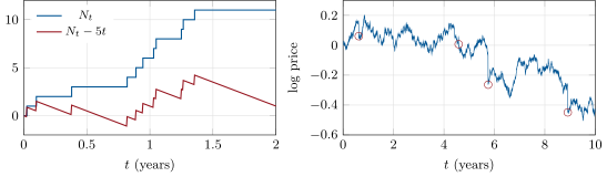
Both are martingales, with ; the increments are independent and centred, and the variance of a Poisson variable is its mean. The compensated process is the jump analogue of Brownian motion: a martingale with quadratic variation , the number of jumps (Figure 6.1, left). Chapter 7 generalises the compensator to rates that depend on the past.
6.2 Itô’s formula with jumps
Definition 6.3 (Jump-diffusion, semimartingale)
A jump-diffusion is , with a compound Poisson process (finitely many jumps on bounded intervals). A semimartingale is a process that is a local martingale plus an adapted process of finite variation, both càdlàg: the widest class of integrators for which stochastic integrals and Itô’s formula work.
Theorem 6.4 (Itô’s formula with jumps)
For a jump-diffusion and ,
Proof. Between two jump times the process is an Itô process and Theorem 3.7 applies; at a jump time the change of is . There are finitely many jumps on , so summing the pieces gives the formula. ∎
The jump term is the exact change, not a Taylor expansion: jumps are not small. With and , ; compensating the last term, is a martingale if and only if , the drift correction that every jump model of One Quant Book 5 carries.
6.3 Lévy processes and the Lévy–Khintchine formula
Definition 6.5 (Lévy process, infinitely divisible distribution)
A Lévy process is a càdlàg process with and independent, stationary increments. A law is an infinitely divisible distribution if for every it is the law of a sum of independent, identically distributed variables.
The law of of a Lévy process is infinitely divisible ( is the sum of increments of length ), and conversely every infinitely divisible law is the law of for some Lévy process. Brownian motion with drift, the Poisson and compound Poisson processes, and their sums are Lévy processes; the general one adds infinitely many small jumps.
Definition 6.6 (Lévy measure, Lévy triplet, characteristic exponent)
The Lévy measure of a Lévy process is , the expected number of jumps per unit time with size in (); it satisfies . The Lévy triplet is : Gaussian variance, Lévy measure and drift. The characteristic exponent is the function with .
Theorem 6.7 (Lévy–Khintchine)
The characteristic exponent of a Lévy process with triplet is
and every triplet with and defines a Lévy process. Moreover decomposes into a Brownian motion with drift, a compound Poisson process of the jumps larger than one, and a square-integrable martingale of the compensated small jumps (Lévy–Itô).
Proof. Admitted here. ∎
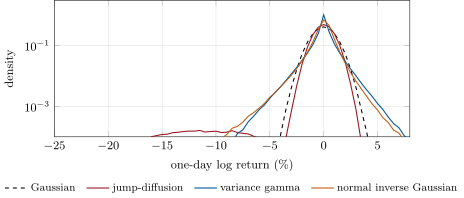
For a compound Poisson process with rate and jump law , and the integral is , up to a drift: the computation is one line of conditioning on . The chapter’s jump-diffusion, with Gaussian jumps, has . Every model of the running project is specified by its exponent (the tutorial’s first listing), and Figure 6.2 compares four of them at one day.
Definition 6.8 (Subordinator)
A subordinator is a Lévy process with nondecreasing paths; running a Brownian motion on it as a clock, , gives a Lévy process whose exponent is the subordinator’s Laplace exponent evaluated at .
The gamma subordinator gives the variance gamma process and the inverse Gaussian one the normal inverse Gaussian process: trading time that runs fast on busy days and slow on quiet ones. One Quant Book 5, chapter 13, defines the pricing models built on them. With the same annual variance as the chapter’s jump-diffusion, they spread their tail differently: the jump-diffusion keeps a Gaussian body and adds a distant bump of crash days, the subordinated models fatten the whole tail smoothly (Figure 6.2).
6.4 Cumulants and the term structure of kurtosis
Definition 6.9 (Cumulant)
The -th cumulant of a random variable is the -th derivative at zero of its cumulant generating function ; is the mean, the variance, the skewness and the excess kurtosis.
Proposition 6.10 (Cumulants of a Lévy process scale with time)
For a Lévy process, . Hence the skewness of decays like and its excess kurtosis like . For Gaussian jumps, is the Gaussian part plus .
Proof. is linear in , and so are its derivatives. For the compound Poisson part the cumulant generating function is , whose -th derivative at zero is . ∎
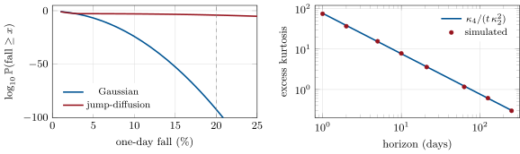
A jump model that explains one-day crashes is close to Gaussian at a month: the kurtosis it needs at one day is diluted by averaging. For the chapter’s calibration the excess kurtosis is 76 at one day and 3.6 at a month (Figure 6.3). Returns measured in markets keep more kurtosis at a month than this law allows, because their volatility itself clusters: the independence of increments, not the jumps, is what fails at longer horizons (chapter 18).
6.5 Tutorial: a characteristic function you can check
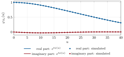
Goal. Specify the chapter’s jump-diffusion by its characteristic exponent, simulate it, and check the exponent, the cumulants and the kurtosis term structure against the paths. End state: Figures 6.1, 6.3 and 6.4 and the calibration of the weekend problem.
The exponents of the running project’s Lévy models.
def psi_bm(u, mu: float, sigma: float):
    u = np.asarray(u, dtype=complex)
    return 1j * mu * u - 0.5 * sigma**2 * u**2


def psi_merton(u, mu: float, sigma: float, lam: float, mu_j: float, sigma_j: float):
    u = np.asarray(u, dtype=complex)
    return psi_bm(u, mu, sigma) + lam * (np.exp(1j * u * mu_j - 0.5 * sigma_j**2 * u**2) - 1)


def psi_kou(u, mu: float, sigma: float, lam: float, p: float, eta1: float, eta2: float):
    u = np.asarray(u, dtype=complex)
    return psi_bm(u, mu, sigma) + lam * (p * eta1 / (eta1 - 1j * u) + (1 - p) * eta2 / (eta2 + 1j * u) - 1)


def psi_vg(u, theta: float, sigma: float, nu: float):
    u = np.asarray(u, dtype=complex)
    return -np.log(1 - 1j * u * theta * nu + 0.5 * sigma**2 * nu * u**2) / nu


def psi_nig(u, alpha: float, beta: float, delta: float):
    u = np.asarray(u, dtype=complex)
    return delta * (np.sqrt(alpha**2 - beta**2) - np.sqrt(alpha**2 - (beta + 1j * u) ** 2))
Listing 6.1. Characteristic exponents: Brownian motion, Gaussian and double-exponential jumps, variance gamma, normal inverse Gaussian. code/firm/levy/firm_levy.py The calibration: bisect on the mean jump size until a fall of 20% is a once-in-fifty-years event, holding the daily variance at .
def calibrate(target_per_day: float = 1 / (EVERY * YEAR)) -> dict:
    """Find the mean jump size mu_j (negative) such that P(day <= -20%) hits the target, with the
    diffusion volatility adjusted so that the daily variance stays SD_DAY^2."""
    def sig_c(mu_j):
        v = SD_DAY**2 - LAM / YEAR * (mu_j**2 + SIG_J**2)
        return math.sqrt(v * YEAR) if v > 0 else float("nan")

    lo, hi = -0.20, 0.0
    for _ in range(80):
        mid = 0.5 * (lo + hi)
        sc = sig_c(mid)
        if math.isnan(sc) or day_tail(DROP, mid, sc) > target_per_day:
            lo = mid
        else:
            hi = mid
    mu_j = 0.5 * (lo + hi)
    return {"mu_j": mu_j, "sig_c": sig_c(mu_j), "tail": day_tail(DROP, mu_j, sig_c(mu_j))}
Listing 6.2. Calibrating the jump size to a tail frequency at fixed variance. code/methods/06-jump-processes/python/qm_jumps.py - Run
problem(),charfn_check()andfig_jumps.py; the numerical cumulants offirm_levy.cumulantsagree with the closed forms to .
What to change next. Replace the Gaussian jumps by double-exponential ones with the same mean and variance and compare the two tails at 20%; simulate variance gamma by subordination and check its kurtosis against at unit time.
6.6 Build: the Lévy toolkit
Purpose. Every jump model of the miniature firm is specified once, by its characteristic exponent, and used three ways: to simulate, to compute moments, and to price by transform (chapter 28).
Interface. psi_bm, psi_merton, psi_kou, psi_vg, psi_nig; cumulants(psi, n_max); merton_cumulants(…); exp_martingale_drift(psi); simulate_merton, simulate_vg, simulate_nig.
Rules. Exponents take complex arguments and follow the series’ convention ; simulations are exact on their grid; the martingale drift is computed from the exponent, never typed.
Acceptance tests. code/firm/levy/tests/: numerical cumulants equal the closed forms; empirical characteristic functions of simulated paths match ; variance gamma and normal inverse Gaussian paths have the moments their exponents give; with the computed drift has constant mean.
Stretch. CGMY and stable exponents; exact simulation of first-passage times for spectrally negative processes.
Sources and further reading
- Federal Reserve History, “Stock Market Crash of 1987”.
- CFA Institute, Enterprising Investor, “Fact file: S&P 500 sigma events”, 2012.
- R. C. Merton, “Option pricing when underlying stock returns are discontinuous”, Journal of Financial Economics 3, 1976.
- S. G. Kou, “A jump-diffusion model for option pricing”, Management Science 48, 2002.
- R. Cont and P. Tankov, Financial Modelling with Jump Processes, Chapman & Hall/CRC, 2004.
6.7 Exercises
Exercise 6.1 ★
Events arrive as a Poisson process at 5 a year. What is the probability of none in a month, and the expected wait for the next one?
Solution
Solution of Exercise 6.1.
; by memorylessness the expected wait is of a year, whatever has happened.
Exercise 6.2 ★
Jumps arrive at 3 a year with sizes . What are the mean and standard deviation of their sum over a year?
Solution
Solution of Exercise 6.2.
Mean ; variance , a standard deviation of 7.75%.
Exercise 6.3 ★
Show that is a martingale and that .
Solution
Solution of Exercise 6.3.
For , is independent of with mean , so ; and .
Exercise 6.4 ★★
For with compound Poisson, write with Theorem 6.4, and find the drift to add to so that is a martingale.
Solution
Solution of Exercise 6.4.
. The jump term has compensator , so the drift added to makes a martingale.
Exercise 6.5 ★★
Jumps arrive at rate 2 with exponential sizes of mean . Write the characteristic exponent of the compound Poisson process and its mean and variance at .
Solution
Solution of Exercise 6.5.
; mean , variance .
Exercise 6.6 ★★
A Lévy model has an excess kurtosis of 76.4 at one day. What does it have at a week of five days and at a year of 252?
Solution
Solution of Exercise 6.6.
at a week and at a year.
Exercise 6.7 ★★★
Coding. With cumulants, compute the first four cumulants of the variance gamma process with , , at unit time, and check them against , , , .
Solution
Solution of Exercise 6.7.
both ways: the finite differences of the cumulant generating function agree with the formulas to about .
Exercise 6.8 ★★★
Find the flaw. “Monthly returns of our index have an excess kurtosis of 1.2, close to Gaussian, so jumps do not matter for our one-day risk.”
Solution
Solution of Exercise 6.8.
In a Lévy model the excess kurtosis falls like : 1.2 at 21 days corresponds to about 25 at one day. Monthly returns average away exactly the jumps that matter for one-day risk; measure the tail at the horizon of the risk.
6.8 Problem: Twenty Standard Deviations
Problem 6.1
Weekend problem — a crash that a diffusion cannot produce
Daily returns of an index have a standard deviation of 0.98%. A risk manager wants a model in which a one-day fall of 20% or more happens once in fifty years of 252 days, and ordinary days keep that variance. The model is a jump-diffusion: jumps at rate a year with sizes , and a diffusion whose volatility makes up the rest of the variance.
Part I — The day.
- How large a fall is 20.98 standard deviations?
- What probability does a Gaussian with that standard deviation give it? (Give .)
- And a fall of exactly 20%?
- What annual volatility does 0.98% a day make?
- Why can re-estimating the volatility not rescue the Gaussian model?
Part II — The jump-diffusion.
- What mean jump size makes a 20% fall a once-in-fifty-years event?
- What diffusion volatility keeps the daily variance at ?
- What share of the variance do the jumps carry?
- What is the probability of a jump on a given day?
- How often does the model produce a fall of 10% or more?
Part III — Cumulants.
- What are the one-day skewness and excess kurtosis?
- What is the excess kurtosis at a month of 21 days?
- Why does it fall like ?
- What drift correction makes a martingale?
- Check the kurtosis at five days against simulation.
Part IV — Judgement.
- Is “once in fifty years” an estimate or a choice?
- What would the model miss that the data show at a month?
- Which options does the calibration matter most for?
- State the named result: the size of the 1987 day under a diffusion, and the jump that makes it rare but possible.
- In one sentence: what does a jump process change that a volatility cannot?
Solution
Solution of Problem 6.1.
1. . 2. . 3. standard deviations: probability . 4. . 5. A Gaussian volatility high enough to make the day plausible would make ordinary days several times more volatile than they are; the tail and the body cannot both fit. 6. . 7. 13.0% a year (12.96%). 8. 31%: out of . 9. . 10. With probability 0.116% a day: once every 3.4 years. 11. Skewness , excess kurtosis 76.4. 12. . 13. Cumulants of a Lévy process are linear in , so . 14. a year, on top of . 15. 15.3 in theory, 15.6 in 400 000 simulated five-day returns. 16. A choice: one such day in the record cannot estimate a frequency; the model encodes a judgement about how often it should be allowed to happen. 17. Volatility clustering: in the data the kurtosis decays more slowly than (chapter 18). 18. Short-dated, far out-of-the-money puts, whose value is almost all jump probability (One Quant Book 5, chapter 13). 19. Named result: twenty standard deviations: the 1987 day was a 21-standard-deviation fall, with Gaussian probability ; jumps at rate 0.5 a year with mean and standard deviation 5%, carrying 31% of the variance, make a fall of 20% a once-in-fifty-years event, at the cost of a one-day excess kurtosis of 76 (3.6 at a month). 20. It changes the shape of the one-day law, putting mass in the tail without raising the variance of ordinary days.
6.9 Interview questions
Interview question 6.1 ★ trader, risk
A model says yesterday’s move was a 20-standard-deviation event. What do you conclude?
Solution
Solution of Interview question 6.1.
That the model, not the market, is wrong: under it the move should never have happened. Check the data first (a bad print, a corporate action), then the model’s assumptions (continuous paths, constant volatility, Gaussian shocks) and the risk numbers that depend on them.
What the interviewer is looking for: model failure, not bad luck.
Interview question 6.2 ★ researcher
Trades arrive as a Poisson process at 2 a second. What is the probability of at least two in a second, and the expected time to the next one?
Solution
Solution of Interview question 6.2.
; half a second, whatever the time since the last trade.
What the interviewer is looking for: Poisson probabilities and memorylessness.
Interview question 6.3 ★★ bank, trader
Why can a delta hedge not remove the risk of a jump?
Solution
Solution of Interview question 6.3.
A delta hedge offsets small moves to first order; a jump is a large move, and the option’s value changes by the full difference , not . With random jump sizes there is one more source of risk than the stock can hedge: the market is incomplete.
What the interviewer is looking for: nonlinearity plus incompleteness.
Interview question 6.4 ★★ researcher
State the Lévy–Khintchine formula and say what each part of the triplet means.
Solution
Solution of Interview question 6.4.
: a drift, the Brownian variance, the expected number of jumps per unit time by size.
What the interviewer is looking for: the three parts and the role of .
Interview question 6.5 ★★ researcher, risk
How does the kurtosis of returns change with the horizon in a Lévy model, and in the data?
Solution
Solution of Interview question 6.5.
Cumulants scale with , so the excess kurtosis falls like and a monthly return is nearly Gaussian. In the data it falls more slowly, because volatility clusters and increments are not independent.
What the interviewer is looking for: and what breaks it.
Interview question 6.6 ★★★ bank, researcher
In a jump-diffusion for a stock under the risk-neutral measure, what must the drift be, and why?
Solution
Solution of Interview question 6.6.
The discounted price must be a martingale: for with , , the jump compensator removing the jumps’ average contribution. Otherwise the model admits arbitrage against the money-market account.
What the interviewer is looking for: the compensator in the drift.