Quantitative Methods · Methods

10Optimal Stopping and Impulse Control

A bank’s treasury desk carries a euro exposure that drifts with its clients’ flows: every payment, every trade finance deal, moves it by a few million. Each hedge ticket costs a fixed amount; carrying the exposure costs a risk charge that grows with its square. Hedging after every client flow wastes fees; never hedging lets the risk grow without bound. The answer is a band: do nothing while the exposure is inside $\pm b$ , trade it back to zero when it touches the edge. With the desk’s numbers the best band is $\pm$ USD 34.6 million, a hedge every three days on average, and the policy costs half as much as hedging once a day at the close; if the ticket fee halves, the band narrows by only 16%, because the optimal band grows with the fourth root of the fee. Deciding when to act is a stopping problem; deciding when and how much to act, repeatedly, is impulse control. This chapter solves both: the Snell envelope in discrete time, free boundaries and smooth pasting in continuous time, impulse control and its no-trade region, and singular control, its limit when costs are proportional.

10.1 Optimal stopping in discrete time: the Snell envelope

Definition 10.1 (Optimal stopping problem, Snell envelope)

Given an adapted, integrable reward process $(G_n)_{n\le N}$ , the optimal stopping problem is to find $\sup_\tau\E[G_\tau]$ over stopping times $\tau \le N$ . Its Snell envelope is defined backward by $U_N = G_N$ and $U_n = \max(G_n, \E_n[U_{n+1}])$ .

Theorem 10.2 (The Snell envelope solves the stopping problem)

$U$ is the smallest supermartingale dominating $G$ ; $U_n = \sup_{\tau \ge n}\E_n[G_\tau]$ ; and $\tau^* = \min\{n : U_n = G_n\}$ is optimal.

Proof. $U_n \ge \E_n[U_{n+1}]$ and $U_n \ge G_n$ by construction. If $Y$ is a supermartingale dominating $G$ , then $Y_N \ge U_N$ and, backward, $Y_n \ge \max(G_n, \E_n[Y_{n+1}]) \ge U_n$ . Up to $\tau^*$ the envelope equals its conditional expectation, so $U_{n\wedge\tau^*}$ is a martingale and $\E[G_{\tau^*}] = \E[U_{\tau^*}] = U_0$ ; any other $\tau$ gives $\E[G_\tau] \le \E[U_\tau] \le U_0$ by optional stopping for the supermartingale. ∎

Definition 10.3 (Continuation region, stopping region)

For a Markov problem with $G_n = g(n, X_n)$ and $U_n = u(n, X_n)$ , the stopping region is $\{(n, x) : u = g\}$ and the continuation region its complement, where waiting is strictly better.

The running project’s solver of chapter 9 computes the Snell envelope by adding the stopping reward to the backward induction: $V_t = \max(\text{stop}, \text{continue})$ . An American option is the best-known stopping problem; One Quant Book 5, chapter 6, prices it and names its boundary. Here the same mathematics decides when to take profit on a trade.

10.2 Free boundaries and variational inequalities

In continuous time, with $X$ a diffusion with generator $\mathcal L$ and a discount rate $r$ , the value $V(x) = \sup_\tau\E_x[e^{-r\tau}g(X_\tau)]$ of a perpetual stopping problem satisfies, where smooth,

\max\bigl(\mathcal LV - rV,\ g - V\bigr) = 0:

in the continuation region $V > g$ and $V$ solves the equation $\mathcal LV = rV$ ; in the stopping region $V = g$ and waiting would not pay, $\mathcal Lg - rg \le 0$ .

Definition 10.4 (Variational inequality, free-boundary problem, smooth pasting)

The display above is a variational inequality. Written as “solve $\mathcal LV = rV$ on an unknown region $D$ with $V = g$ on its boundary”, it is a free-boundary problem: the boundary $\partial D$ is part of the solution. The extra condition that fixes it, $V' = g'$ on $\partial D$ where $g$ is smooth, is smooth pasting (or smooth fit).

Proposition 10.5 (Taking profit on a drifting position)

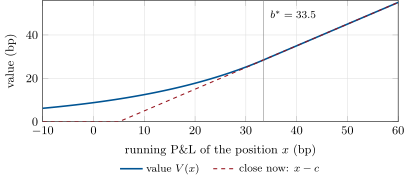
Let $X_t = x + \mu t + \sigma W_t$ be the running P&L of a position, $c$ the cost of closing it, and $r > 0$ a discount rate. The optimal rule for $\sup_\tau\E[e^{-r\tau}(X_\tau - c)]$ closes the first time $X$ reaches $b^* = c + 1/\theta$ , where $\theta > 0$ solves $\tfrac12\sigma^2\theta^2 + \mu\theta - r = 0$ , and $V(x) = (b^* - c)e^{\theta(x - b^*)}$ for $x < b^*$ .

Proof. For a threshold $b$ , $\E_x[e^{-r\tau_b}] = e^{\theta(x - b)}$ for $x < b$ , since $e^{-rt + \theta X_t}$ is a martingale exactly when $\theta$ solves the quadratic; so the value of the $b$ -rule is $(b - c)e^{\theta(x - b)}$ , maximised over $b$ at $b = c + 1/\theta$ . There $V'(b^*) = \theta(b^* - c) = 1 = g'(b^*)$ : smooth pasting. On $x \ge b^*$ , $V = x - c$ and $\mathcal Lg - rg = \mu - r(x - c) \le 0$ because $x - c \ge 1/\theta \ge \mu/r$ , so the variational inequality holds and a verification argument as in chapter 9 applies. ∎

With $\mu = 0.5$ and $\sigma = 2$ basis points a day, a closing cost of 5 bp and $r = 2\%$ a day, $\theta = 0.0351$ and $b^* = 33.5$ bp. Backward induction on a grid, observing the position once a day, stops at 32.2 bp and values the position at 8.79 bp at zero against 8.80 (Figure 10.1): the daily grid stops a little earlier, by about the overshoot $0.5826\,\sigma\sqrt{\Delta t} = 1.2$ bp of chapter 2.

Taking profit on a drifting position (= 0.5, = 2 bp a day, closing cost 5 bp, discount 2% a day). The value of waiting (solid) lies above the value of closing now (dashed) until b* = c + 1/, where it meets it with the same slope: smooth pasting. Data: closed form, checked by the chapter’s grid solver. — **Figure 10.1.** Taking profit on a drifting position ( $\mu = 0.5$ , $\sigma = 2$ bp a day, closing cost 5 bp, discount 2% a day). The value of waiting (solid) lies above the value of closing now (dashed) until $b^* = c + 1/\theta$ , where it meets it with the same slope: smooth pasting. Data: closed form, checked by the chapter’s grid solver.

10.3 Impulse control and no-trade regions

Definition 10.6 (Impulse control, quasi-variational inequality)

Impulse control acts on a state by discrete interventions: at stopping times $\tau_1 < \tau_2 < \dots$ it moves $X$ by jumps $\xi_i$ , each paying a cost with a fixed part $K > 0$ . Its value function satisfies a quasi-variational inequality: $\max(\mathcal LV - rV - f,\ \mathcal MV - V) = 0$ (for a cost-minimisation, with signs reversed), where $\mathcal MV(x) = \sup_\xi\{V(x + \xi) - K - \text{cost}(\xi)\}$ is the value of acting now: the obstacle depends on the unknown $V$ itself.

Definition 10.7 (No-trade region)

The no-trade region of a trading or hedging policy is the set of states in which it does not trade; for one exposure it is an interval $(-b, b)$ , and a band policy trades back to $\pm a$ when the exposure reaches $\pm b$ .

For the desk, let the exposure move as $\sigma W_t$ between hedges, charge $\gamma X_t^2$ per unit time for carrying it, and charge $K$ per hedge ticket plus $c$ per unit traded.

Proposition 10.8 (The cost of a band policy)

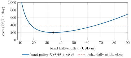
The long-run average cost of the band policy $(a, b)$ is

C(a, b) = \Bigl(K + c(b - a) + \frac{\gamma(b^4 - a^4)}{6\sigma^2}\Bigr)\frac{\sigma^2}{b^2 - a^2}.

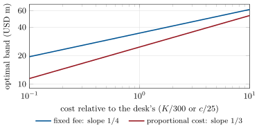
With a fixed cost only ( $c = 0$ ) the optimal reset is $a = 0$ , and $C(0, b) = K\sigma^2/b^2 + \gamma b^2/6$ is minimised at

b^* = \Bigl(\frac{6K\sigma^2}{\gamma}\Bigr)^{1/4}, \qquad C^* = 2\sqrt{K\sigma^2\gamma/6},

where the fees and the risk charge each contribute half.

Proof. A cycle runs from $\pm a$ to the first exit of $(-b, b)$ . By Dynkin’s formula (chapter 4), $m(x) = \E_x[\tau]$ and $f(x) = \E_x\int_0^\tau X_t^2\,dt$ solve $\tfrac12\sigma^2m^{\prime\prime} = -1$ and $\tfrac12\sigma^2f^{\prime\prime} = -x^2$ with zero boundary values: $m(x) = (b^2 - x^2)/\sigma^2$ and $f(x) = (b^4 - x^4)/(6\sigma^2)$ . Each cycle costs $K + c(b - a) + \gamma f(a)$ ; by the renewal–reward theorem the average cost is the expected cost per cycle over the expected cycle length. With $c = 0$ , $\partial_bC = 0$ gives $b^4 = 6K\sigma^2/\gamma$ , and substituting gives $C^*$ with equal parts. ∎

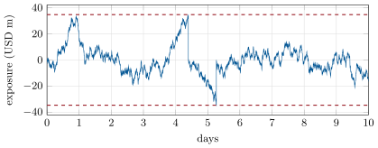
With $\sigma = 20$ (USD millions per square-root day), $\gamma = \text{USD}~0.5$ per (USD million) $^2$ per day and $K = \text{USD}~300$ , $b^* = 34.6$ million and $C^* = \text{USD}~200$ a day, with a hedge every $b^{*2}/\sigma^2 = 3$ days on average (Figures 10.2 and 10.3). Hedging once a day at the close instead costs $K + \gamma\sigma^2/2 = 400$ a day. The cost curve is flat near its minimum and steep toward small bands: a band of 10 million costs 1 208 a day.

Ten simulated days of the desk’s exposure under the optimal band ± 34.6 million (dashed): client flows move it freely inside the no-trade region, and each touch of the band triggers a hedge back to zero. Data: the chapter’s tutorial, seeded. — **Figure 10.2.** Ten simulated days of the desk’s exposure under the optimal band $\pm 34.6$ million (dashed): client flows move it freely inside the no-trade region, and each touch of the band triggers a hedge back to zero. Data: the chapter’s tutorial, seeded.

Average daily cost of the band policy against the band’s half-width, for the desk’s numbers (K = 300, = 20, = 0.5): minimum USD 200 at b* = 34.6 million (dot), half the cost of hedging once a day. Data: closed form, checked by simulation in the tutorial. — **Figure 10.3.** Average daily cost of the band policy against the band’s half-width, for the desk’s numbers ( $K = 300$ , $\sigma = 20$ , $\gamma = 0.5$ ): minimum USD 200 at $b^* = 34.6$ million (dot), half the cost of hedging once a day. Data: closed form, checked by simulation in the tutorial.

10.4 Singular control and reflection

When the cost is proportional only ( $K = 0$ ), small trades cost little, and the optimal policy trades continuously but only at the boundary.

Definition 10.9 (Singular control, reflected Brownian motion)

A singular control acts through a process of finite variation that increases only on a set of times of Lebesgue measure zero. Reflected Brownian motion on $[-b, b]$ is $X = \sigma W + L - U$ , with $L$ and $U$ nondecreasing, increasing only when $X = -b$ and $X = b$ respectively: the minimal pushing that keeps $X$ in the interval.

Reflected Brownian motion on $[-b, b]$ has the uniform stationary law, so $\E[X^2] = b^2/3$ , and its boundaries push at a total long-run rate of $\sigma^2/(2b)$ (apply Itô’s formula to $X^2$ : the drift $\sigma^2$ is balanced by $2b$ times the pushing rate). The average cost is $c\sigma^2/(2b) + \gamma b^2/3$ , minimised at

b^* = \Bigl(\frac{3c\sigma^2}{4\gamma}\Bigr)^{1/3}:

the cube-root law for proportional costs, against the fourth root for fixed costs (Figure 10.4). With $c = \text{USD}~25$ per million (a quarter of a basis point), $b^* = 24.7$ million and the cost is USD 304 a day. With both costs, the optimal band triggers at 42.4 million and trades back to 12.8 million, not to zero, at USD 418 a day: the fixed fee makes trades large, the proportional cost makes them stop short. Davis and Norman (1990) solved the portfolio version, a no-trade region around the Merton fraction of chapter 9.

**Figure 10.4.** Optimal band against the size of the trading cost, on log scales: with a fixed fee per ticket the band grows like the fourth root of the fee, with a proportional cost like the cube root. A hundredfold change in cost moves the bands by factors of 3.2 and 4.6. Data: closed forms, the chapter’s tutorial.

10.5 Tutorial: the hedging band

Goal. Compute the desk’s optimal band, check it by simulating the exposure, find the combined band with fixed and proportional costs, and solve the take-profit problem by smooth pasting and on a grid. End state: Figures 10.2, 10.3, 10.4 and 10.1 and the numbers of the weekend problem.

The band’s cost by renewal–reward, and the two closed-form optima.

def band_cost(b: float, a: float, sigma: float, gamma: float, K: float, c: float = 0.0) -> float:
    """Average cost per unit time: [K + c (b - a) + gamma (b^4 - a^4) / (6 sigma^2)] sigma^2 / (b^2 - a^2).

    A cycle starts at +-a and ends when |X| = b; E[cycle length] = (b^2 - a^2) / sigma^2 and
    E[int X^2 dt] = (b^4 - a^4) / (6 sigma^2) solve (1/2) sigma^2 f'' = -1 and -x^2 with f(+-b) = 0."""
    if not 0 <= a < b:
        return math.inf
    per_cycle = K + c * (b - a) + gamma * (b**4 - a**4) / (6 * sigma**2)
    return per_cycle * sigma**2 / (b**2 - a**2)


def reflect_cost(b: float, sigma: float, gamma: float, c: float) -> float:
    """Reflected Brownian motion on [-b, b]: uniform stationary law, E[X^2] = b^2 / 3, and the
    boundaries push at total rate sigma^2 / (2 b)."""
    return c * sigma**2 / (2 * b) + gamma * b**2 / 3


def optimal_fixed_band(sigma: float, gamma: float, K: float) -> tuple[float, float]:
    b = (6 * K * sigma**2 / gamma) ** 0.25
    return b, band_cost(b, 0.0, sigma, gamma, K)


def optimal_proportional_band(sigma: float, gamma: float, c: float) -> tuple[float, float]:
    b = (3 * c * sigma**2 / (4 * gamma)) ** (1 / 3)
    return b, reflect_cost(b, sigma, gamma, c)

Listing 10.1. The average cost of a band policy, of reflection, and the fourth- and cube-root bands. code/firm/impulse/firm_impulse.py

The stopping threshold by smooth pasting.

def stop_threshold_drift(mu: float, sigma: float, r: float, cost: float) -> tuple[float, float]:
    """Stop X_t = x + mu t + sigma W_t to collect X - cost, discounting at r. For x below the threshold
    V(x) = (b - cost) exp(theta (x - b)) with theta the positive root of sigma^2 th^2 / 2 + mu th - r = 0;
    smooth pasting V'(b) = 1 gives b* = cost + 1 / theta. Returns (b*, theta)."""
    theta = (-mu + math.sqrt(mu * mu + 2 * r * sigma * sigma)) / (sigma * sigma)
    return cost + 1 / theta, theta

Listing 10.2. The take-profit threshold for a drifting position. code/firm/impulse/firm_impulse.py

Run problem(), dp_stopping_check() and fig_bands.py; the simulation of 20 000 days at 390 checks a day gives USD 197 a day for the optimal band, and 200 with checks four times as frequent.

What to change next. Make the client flows mean-revert (the exposure an Ornstein–Uhlenbeck process) and find how the band widens; hedge two correlated currencies with one band on their risk-weighted combination.

10.6 Build: hedging bands

Purpose. Decide when the firm’s hedgers, rebalancers and inventory managers trade: every recurring hedge goes through a band whose width is computed, not guessed.

Interface. band_cost(b, a, sigma, gamma, K, c); reflect_cost(b, sigma, gamma, c); optimal_fixed_band; optimal_proportional_band; optimal_band(sigma, gamma, K, c) returning $(a^*, b^*, C^*)$ ; simulate_band; stop_threshold_drift(mu, sigma, r, cost); golden.

Rules. Units stated at the call site (exposure, time, currency); the closed forms are used where they exist and checked by simulation in the tests; the combined band is searched over both the trigger and the reset.

Acceptance tests. code/firm/impulse/tests/: the renewal formula against simulation; the fourth- and cube-root laws; the numerical optimum reduces to the closed forms when one cost vanishes; smooth pasting holds at the stopping threshold.

Stretch. Mean-reverting exposures; several currencies with a correlation matrix; the Davis–Norman portfolio no-trade region.

Sources and further reading

J. L. Snell, “Applications of martingale system theorems”, Transactions of the AMS 73, 1952.
G. M. Constantinides and S. F. Richard, “Existence of optimal simple policies for discounted-cost inventory and cash management in continuous time”, Operations Research 26, 1978.
M. H. A. Davis and A. R. Norman, “Portfolio selection with transaction costs”, Mathematics of Operations Research 15, 1990.
A. E. Whalley and P. Wilmott, “An asymptotic analysis of an optimal hedging model for option pricing with transaction costs”, Mathematical Finance 7, 1997.
G. Peskir and A. Shiryaev, Optimal Stopping and Free-Boundary Problems, Birkhäuser, 2006.

10.7 Exercises

Exercise 10.1 ★

With $K = 300$ , $\sigma = 20$ and $\gamma = 0.5$ , what are the optimal band, its daily cost and the average number of hedges a day?

Solution

Solution of Exercise 10.1.

$b^* = (6 \times 300 \times 400/0.5)^{1/4} = 34.6$ million; $C^* = 2\sqrt{300 \times 400 \times 0.5/6} = 200$ dollars a day; $\sigma^2/b^{*2} = 1/3$ hedge a day, one every three days.

Exercise 10.2 ★

On the two-step tree of Figure 1.1, compute the Snell envelope of $G_n = (S_n - 100)^+$ and say where it is optimal to stop.

Solution

Solution of Exercise 10.2.

$U_2 = G_2 = (2, 0, 0)$ at $S_2 = 102, 100, 98$ . $U_1 = \max(1, 1) = 1$ at 101 and $\max(0, 0) = 0$ at 99; $U_0 = \max(0, 0.5) = 0.5$ . At time 0 continue ( $U > G$ ); at time 1 stopping is optimal (at 101 exactly indifferent, at 99 nothing is lost).

Exercise 10.3 ★

Is “the day the exposure reaches its largest absolute value this month” a valid time to hedge in the sense of this chapter?

Solution

Solution of Exercise 10.3.

No: whether it is the largest of the month is known only at the month’s end, so it is not a stopping time, and no policy can hedge there.

Exercise 10.4 ★★

If the ticket fee doubles, by how much do the optimal band and its cost change? And if the flow volatility doubles?

Solution

Solution of Exercise 10.4.

Doubling $K$ : band $\times 2^{1/4} = 1.19$ (41.2 million), cost $\times\sqrt2$ (283 dollars). Doubling $\sigma$ : band $\times\sqrt2$ (49.0 million), cost $\times 2$ (400 dollars).

Exercise 10.5 ★★

With only a proportional cost of USD 25 per million, what are the reflecting band and its cost?

Solution

Solution of Exercise 10.5.

$b^* = (3 \times 25 \times 400/2)^{1/3} = 24.7$ million; cost $25 \times 400/49.3 + 0.5 \times 24.7^2/3 = 304$ dollars a day.

Exercise 10.6 ★★

Derive $b^* = c + 1/\theta$ in Proposition 10.5 from smooth pasting alone, and evaluate it for $\mu = 0.5$ , $\sigma = 2$ , $r = 0.02$ , $c = 5$ .

Solution

Solution of Exercise 10.6.

Below the threshold $V(x) = Ae^{\theta x}$ (the solution of $\mathcal LV = rV$ that stays bounded as $x \to -\infty$ ); value matching $Ae^{\theta b} = b - c$ and smooth pasting $A\theta e^{\theta b} = 1$ give $\theta(b - c) = 1$ . With the numbers, $\theta = (-0.5 + \sqrt{0.25 + 0.16})/4 = 0.0351$ and $b^* = 5 + 28.5 = 33.5$ bp.

Exercise 10.7 ★★★

Coding. Simulate the desk’s exposure with the optimal band, checking it 390 and then 1 560 times a day, and compare the average cost with the formula. Why is the discretely checked band cheaper?

Solution

Solution of Exercise 10.7.

197.5 dollars a day at 390 checks and 199.6 at 1 560, against 200. Checked discretely, the exposure overshoots the band before a hedge, so cycles last a little longer and there are fewer tickets; the extra risk charge of the overshoot is smaller than the fees saved, and the gap closes like $\sqrt{\Delta t}$ .

Exercise 10.8 ★★★

Find the flaw. “We hedge as soon as the exposure exceeds 10 million: a tighter band means less risk, and less risk is always better.”

Solution

Solution of Exercise 10.8.

At $b = 10$ the policy costs $300 \times 400/100 + 0.5 \times 100/6 = 1\,208$ dollars a day, six times the optimum: the fees of hedging a dozen times a day dwarf the risk they remove. Risk and fees must be traded off; less risk is not free.

10.8 Problem: The Hedging Band

Problem 10.1

Weekend problem — when to hedge a drifting exposure

A treasury desk’s currency exposure $X$ moves with client flows as $\sigma W_t$ , $\sigma = 20$ million per square-root day. Carrying it costs $\gamma X^2$ a day with $\gamma = 0.5$ dollar per (million) $^2$ ; a hedge ticket costs $K = 300$ dollars; later, trading also costs $c = 25$ dollars per million.

Part I — The fixed fee.

Write the average cost of the band policy that hedges to zero at $\pm b$ .
What is the optimal half-width?
What does it cost a day?
How often does the desk hedge?
What does hedging once a day at the close cost, and what is the band’s saving?

Part II — Scaling.

If the fee halves, what are the new band and cost?
If the flow volatility doubles?
What share of the optimal cost is the risk charge?
What does simulation at 390 and at 1 560 checks a day give?
Why does the discretely checked band come out slightly cheaper?

Part III — Proportional costs.

With the proportional cost only, what are the band and the cost?
With both costs, what are the trigger, the reset and the cost?
Why does the desk no longer trade back to zero?
What distinguishes the singular control of item 11 from the impulse control of item 12?
Solve the take-profit problem of Proposition 10.5 with the chapter’s numbers, in closed form and on a daily grid.

Part IV — Judgement.

Is a quadratic risk charge a sensible model of the desk’s risk?
If client flows mean-revert, should the band be wider or narrower?
Why should the desk net its currencies before banding them?
State the named result: the optimal band and its scaling with the fee.
In one sentence: why is doing nothing inside a band optimal?

Solution

Solution of Problem 10.1.

1. $C(b) = K\sigma^2/b^2 + \gamma b^2/6$ . 2. $b^* = (6K\sigma^2/\gamma)^{1/4} = 34.6$ million. 3. 200 dollars a day. 4. Every three days on average. 5. $300 + 0.5 \times 400/2 = 400$ dollars a day: the band saves 50%. 6. 29.1 million (16% narrower) and 141 dollars a day. 7. 49.0 million and 400 dollars a day. 8. Half: at the optimum fees and risk charge are equal. 9. 197.5 and 199.6 dollars a day. 10. Discrete checks let the exposure overshoot the band, lengthening cycles and saving tickets. 11. 24.7 million and 304 dollars a day. 12. Trigger 42.4 million, reset 12.8 million, 418 dollars a day. 13. Every million traded costs 25 dollars, so stopping short of zero saves proportional cost, and the next cycle, starting closer to the band, is still long enough to amortise the fixed fee. 14. Singular control trades infinitesimally, only when the exposure touches the band, with total traded amount finite; impulse control makes finitely many discrete trades, each paying the fixed fee. 15. $b^* = 33.5$ bp in closed form; the daily grid stops at 32.2 bp and values the position at zero at 8.79 bp against 8.80. 16. As a variance charge, yes: the P&L variance of an open exposure is proportional to $X^2$ . A charge proportional to $|X|$ (a VaR-type limit) changes the exponents of the band laws. 17. Wider: flows that offset themselves make waiting cheaper, since part of the exposure disappears without a trade. 18. Correlated exposures partly offset; banding the net risk hedges less often than banding each currency. 19. Named result: the hedging band: the optimal no-trade band is $\pm(6K\sigma^2/\gamma)^{1/4} = \pm 34.6$ million, costing 200 dollars a day, half the cost of daily hedging; the band grows like the fourth root of the ticket fee (16% narrower if the fee halves). 20. Inside the band the risk removed by a hedge is worth less than the fee it costs, and waiting keeps the option to hedge a larger exposure for the same fee.

10.9 Interview questions

Interview question 10.1 ★ trader, bank

You must hedge an exposure that drifts with client flows, and each hedge costs a fixed fee. Describe the optimal policy.

Solution

Solution of Interview question 10.1.

A band: do nothing while the exposure is within $\pm b$ , trade back to zero at the edge, with $b = (6K\sigma^2/\gamma)^{1/4}$ for a fee $K$ , flow volatility $\sigma$ and risk charge $\gamma X^2$ . It equalises fees and risk charge.

What the interviewer is looking for: no-trade region, the trade-off, and the scaling.

Interview question 10.2 ★★ researcher

What is smooth pasting, and why should the value function meet the payoff with the same slope?

Solution

Solution of Interview question 10.2.

At the optimal boundary the value of waiting and of stopping agree (value matching) and so do their slopes. If the value of waiting met the payoff at an angle, moving the boundary slightly would raise the value: the threshold would not be optimal.

What the interviewer is looking for: first-order optimality of the boundary.

Interview question 10.3 ★★ researcher, trader

Why does an optimal hedging band scale with the fourth root of a fixed fee but the cube root of a proportional cost?

Solution

Solution of Interview question 10.3.

With a fixed fee, the cost per unit time is fee times hedge frequency $\sigma^2/b^2$ plus a risk charge $\propto b^2$ : $b^4 \propto K$ . With a proportional cost, trading happens at rate $\sigma^2/b$ in size at the boundary, so the cost is $c\sigma^2/b$ plus $\propto b^2$ : $b^3 \propto c$ .

What the interviewer is looking for: how often and how much one trades as a function of $b$ .

Interview question 10.4 ★★ bank, researcher

What is the Snell envelope, and how does it relate to pricing an American option?

Solution

Solution of Interview question 10.4.

The smallest supermartingale dominating the reward process, computed backward as the maximum of stopping now and the expected value of continuing; the first time it equals the reward is optimal. The price of an American option is the Snell envelope of its discounted payoff under the risk-neutral measure (One Quant Book 5, chapter 6).

What the interviewer is looking for: the backward recursion and its optimality.

Interview question 10.5 ★★ developer

Implement a band hedger that must not trade back and forth when the exposure sits on the band. What goes into the design?

Solution

Solution of Interview question 10.5.

Trade to a reset level strictly inside the band, never to the band itself, so a hedge cannot immediately trigger another; measure the exposure net of pending hedges; debounce noisy exposure feeds; cap the number of hedges per interval; log each decision with the exposure and the band in force; compute the band from current inputs, not a constant.

What the interviewer is looking for: hysteresis, in-flight orders, and auditability.

Interview question 10.6 ★★★ researcher

For a Brownian motion with variance $\sigma^2$ started at 0, compute $\E\int_0^\tau X_t^2\,dt$ , where $\tau$ is the first exit from $(-b, b)$ .

Solution

Solution of Interview question 10.6.

$f(x) = \E_x\int_0^\tau X^2\,dt$ solves $\tfrac12\sigma^2f^{\prime\prime} = -x^2$ with $f(\pm b) = 0$ , so $f(x) = (b^4 - x^4)/(6\sigma^2)$ and $f(0) = b^4/(6\sigma^2)$ .

What the interviewer is looking for: Dynkin’s formula and a boundary-value problem.

Terms defined in this chapter

See all 2333 terms in the glossary