Quantitative Methods · Methods

18Volatility Models

A risk report measures each currency’s volatility by the equally weighted standard deviation of its last 250 daily returns. On 11 November 2022 the euro rose 3.5% against the dollar: it was the first ECB reference rate (set around 14:10 CET) after the US consumer price index for October, released at 8:30 New York time on 10 November, showed annual inflation slowing to 7.7%. At the close of 2 November 2023, 250 fixings later, that return leaves the window, and the EUR/USD volatility the report carries into the next day falls from 0.538% to 0.496%, by 7.8%, on a day when the euro rose 1.2%. A model that let old news fade gradually would have reported a rise. This chapter is about the models that do: the ARCH and GARCH family and their exponentially weighted special case, realised variance from intraday data and the heterogeneous autoregression that forecasts it, and the loss functions and tests that decide which forecast is better when the truth is never observed.

18.1 The conditional-heteroskedasticity family

Definition 18.1 (Volatility clustering, conditional heteroskedasticity)

Volatility clustering is the tendency of large returns, of either sign, to follow large returns, and small ones small: squared returns are positively autocorrelated although returns are nearly not. A return series has conditional heteroskedasticity when its variance given the past, $h_t = \Var(r_t \mid \mathcal F_{t-1})$ , varies over time.

Definition 18.2 (ARCH and GARCH models, volatility persistence)

In an ARCH model (Engle, 1982), $r_t = \sqrt{h_t}z_t$ with iid standardised $z_t$ and $h_t = \omega + \sum_{i=1}^q\alpha_ir_{t-i}^2$ . The GARCH model (Bollerslev, 1986) adds lagged variances; GARCH(1,1) is $h_t = \omega + \alpha r_{t-1}^2 + \beta h_{t-1}$ with $\omega > 0$ , $\alpha, \beta \ge 0$ . Its volatility persistence is $\alpha + \beta$ , the rate at which a variance shock decays.

Proposition 18.3 (Stationarity and half-life of GARCH(1,1))

If $\alpha + \beta < 1$ , the GARCH(1,1) return is weakly stationary with unconditional variance $\bar h = \omega/(1 - \alpha - \beta)$ , and the forecast of the variance $k$ days ahead is $\E_t[h_{t+k}] = \bar h + (\alpha + \beta)^{k-1}(h_{t+1} - \bar h)$ . A shock to the variance halves in $\ln\frac12/\ln(\alpha + \beta)$ days.

Proof. $\E_t[r_{t+k}^2] = \E_t[h_{t+k}]$ , so $\E_t[h_{t+k+1}] = \omega + (\alpha + \beta)\E_t[h_{t+k}]$ , a linear recursion with fixed point $\bar h$ and rate $\alpha + \beta$ . Taking unconditional expectations gives $\E[r^2] = \bar h$ when $\alpha + \beta < 1$ . ∎

The parameters are estimated by maximising the likelihood of the returns given the recursion, with normal or Student- $t$ innovations. When the normal likelihood is used although the innovations are not normal, the estimator is a quasi-maximum likelihood estimator: it remains consistent and asymptotically normal under regularity conditions, and its standard errors must be the sandwich of chapter 11.

Definition 18.4 (EWMA volatility)

The EWMA volatility with decay $\lambda$ is $h_t = \lambda h_{t-1} + (1 - \lambda)r_{t-1}^2$ : an exponentially weighted average of past squared returns. RiskMetrics (1996) set $\lambda = 0.94$ for daily data.

EWMA is GARCH(1,1) with $\omega = 0$ , $\alpha = 1 - \lambda$ and $\beta = \lambda$ : integrated, $\alpha + \beta = 1$ , so it has no unconditional variance to revert to and its forecast at every horizon is today’s value. With $\lambda = 0.94$ a return’s weight halves in 11 days. The equally weighted window is the other extreme: every return in the window has the same weight, and then none.

Definition 18.5 (Leverage effect, GJR-GARCH model)

The leverage effect is the tendency of volatility to rise more after falls than after rises of the same size, strong for equity indices. The GJR-GARCH model (Glosten, Jagannathan and Runkle, 1993) captures it with $h_t = \omega + (\alpha + \gamma\mathbf 1_{r_{t-1} < 0})r_{t-1}^2 + \beta h_{t-1}$ ; its persistence is $\alpha + \beta + \gamma/2$ for symmetric innovations.

Fitted to 7 098 daily EUR/USD returns (1999–2026, in percent), the three models give:

	$\omega$	$\alpha$	$\beta$	$\gamma$	$\nu$	$\alpha + \beta + \gamma/2$	half-life
GARCH, normal	0.0010	0.029 (0.003)	0.968 (0.004)	—	—	0.9973	255
GARCH, Student $t$	0.0007	0.030 (0.003)	0.968 (0.003)	—	7.2 (0.6)	0.9984	445
GJR, Student $t$	0.0006	0.027 (0.005)	0.969 (0.004)	0.006 (0.005)	7.2 (0.6)	0.9986	482

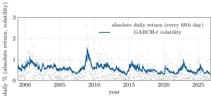
with sandwich standard errors in parentheses. The Student- $t$ likelihood is higher by 141 log points for one extra parameter; the asymmetry is not significant (a currency pair has no natural “down” direction, unlike an equity index); and the persistence is so close to one that a shock to EUR/USD volatility takes well over a year to halve: the long memory of volatility of chapter 17, seen through a short-memory model (Figure 18.1).

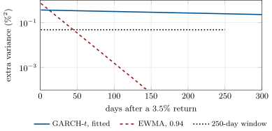
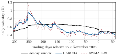
Daily EUR/USD absolute returns and the conditional volatility of the fitted GARCH(1,1) with Student-t innovations, 1999–2026. The clusters (2000, 2008–2009, 2011, 2015, 2022) are what the model’s persistence of 0.9984 describes. Data: ECB euro reference rates (source: ECB statistics). — **Figure 18.1.** Daily EUR/USD absolute returns and the conditional volatility of the fitted GARCH(1,1) with Student- $t$ innovations, 1999–2026. The clusters (2000, 2008–2009, 2011, 2015, 2022) are what the model’s persistence of 0.9984 describes. Data: ECB euro reference rates (source: ECB statistics).

The three estimators treat one large return very differently (Figure 18.2). A 3.5% day adds to the variance forecast an amount that decays at 0.9984 a day under the fitted GARCH, at 0.94 a day under EWMA, and not at all under the window, which carries it undiminished for 250 days and then drops it at once. That drop is the hook’s ghost (Figure 18.3): on the day it happened, the window’s volatility fell 7.8%, while the GARCH volatility rose from 0.424% to 0.465% and the EWMA from 0.410% to 0.490%, both reacting to the day’s 1.2% move.

**Figure 18.2.** How long one 3.5% daily return stays in each variance forecast (the extra variance over a background of 0.5% days). GARCH lets it decay slowly (half-life 445 days), EWMA quickly (11 days), and the equally weighted window keeps it whole for 250 days and then drops it in one step. Data: the chapter’s tutorial, from the fitted parameters.

Figure 18.3. EUR/USD volatility forecasts around the day the return of 11 November 2022 left the 250-day window (day 0, 2 November 2023). The window jumps up by the same amount when the return enters (day

-250

) and falls by 7.8% when it leaves; the GARCH and EWMA forecasts respond to the market, not to the calendar. Data: ECB euro reference rates (source: ECB statistics).

18.2 Realised volatility

Definition 18.6 (Integrated variance, realised variance)

If the log price follows $dX_t = \mu_t\,dt + \sigma_t\,dW_t$ , the integrated variance of day $t$ is $\mathrm{IV}_t = \int_{t-1}^t\sigma_s^2\,ds$ . The realised variance is the sum of the day’s squared intraday returns, $\mathrm{RV}_t = \sum_{j=1}^m r_{t,j}^2$ over $m$ intervals.

Proposition 18.7 (Realised variance converges to integrated variance)

Without microstructure noise, $\mathrm{RV}_t \to \mathrm{IV}_t$ in probability as $m \to \infty$ ; if $\sigma$ is constant within the day, $\mathrm{RV}_t/\mathrm{IV}_t$ has mean one and standard deviation $\sqrt{2/m}$ .

Proof. $\mathrm{RV}_t$ is the discretised quadratic variation of $X$ , which converges to $\int\sigma^2$ (chapter 3). With constant $\sigma$ , each $r_{t,j} \sim \mathcal N(0, \mathrm{IV}_t/m)$ (the drift is negligible at this scale), so $m\,\mathrm{RV}_t/\mathrm{IV}_t$ is $\chi^2_m$ , with mean $m$ and variance $2m$ . ∎

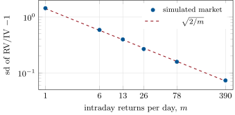
A squared daily return is realised variance with $m = 1$ : an unbiased but very noisy measure of the day’s variance, with a relative error of $\sqrt2 = 141\%$ . Five-minute returns over a 6.5-hour session ( $m = 78$ ) cut it to 16%. The chapter’s simulated market has three volatility components (daily AR coefficients 0.3, 0.9 and 0.99); the measured relative errors are 144%, 16% and 7.3% for $m = 1$ , 78 and 390, against the theory’s 141%, 16% and 7.2% (Figure 18.4). In real markets the gain stops at the frequency where bid-ask bounce and discreteness dominate the returns, the subject of chapter 21.

Relative error of realised variance as a measure of integrated variance, against the number of intraday returns (1 = daily squared return, 78 = five minutes over 6.5 hours, 390 = one minute), in a simulated three-component stochastic-volatility market without microstructure noise, and the theory √2/m. Data: the chapter’s tutorial, seeded. — **Figure 18.4.** Relative error of realised variance as a measure of integrated variance, against the number of intraday returns (1 = daily squared return, 78 = five minutes over 6.5 hours, 390 = one minute), in a simulated three-component stochastic-volatility market without microstructure noise, and the theory $\sqrt{2/m}$ . Data: the chapter’s tutorial, seeded.

18.3 Heterogeneous autoregressive models

Definition 18.8 (HAR model)

The HAR model (Corsi, 2009) regresses tomorrow’s realised variance on today’s, on the average of the last five days and on the average of the last twenty-two: $\mathrm{RV}_{t+1} = b_0 + b_d\mathrm{RV}_t + b_w\mathrm{RV}_t^{(5)} + b_m\mathrm{RV}_t^{(22)} + e_{t+1}$ .

Three horizons of averaging, fitted by least squares, reproduce the slow hyperbolic-looking decay of volatility autocorrelations with an AR model of order 22 restricted to three parameters: long memory approximated by a cascade of short ones. On 2 000 days of the simulated market the fit is $b_d = 0.35$ , $b_w = 0.27$ , $b_m = 0.20$ with $R^2 = 0.37$ ; over the next 1 000 days its forecasts beat an AR(1) on realised variance (QLIKE $-0.479$ against $-0.473$ , Diebold–Mariano statistic $-4.5$ ) and are closer to the true integrated variance (mean squared error 0.0073 against 0.0079).

18.4 Forecasting and evaluation

The variance of a day is never observed, only a proxy: a squared return, or a realised variance. A loss function compares a forecast $h$ with the proxy $\hat\sigma^2$ ; Patton (2011) showed that the ranking of forecasts is preserved under a noisy but unbiased proxy only for a family of losses that includes the squared error and QLIKE.

Definition 18.9 (QLIKE loss, Mincer–Zarnowitz regression, Diebold–Mariano test)

The QLIKE loss is $\hat\sigma^2/h + \ln h$ (up to terms that do not involve $h$ ), the negative Gaussian log-likelihood of the proxy’s return: minimised in expectation by $h = \E[\hat\sigma^2]$ and heavier on under-prediction than on over-prediction. The Mincer–Zarnowitz regression (1969) of the proxy on the forecast, $\hat\sigma^2_t = a + bh_t + e_t$ , tests unbiasedness ( $a = 0$ , $b = 1$ ). The Diebold–Mariano test (1995) of equal accuracy divides the mean loss difference of two forecasts by its HAC standard error.

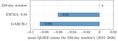
On EUR/USD, the GARCH- $t$ is refitted on 1999–2014 only (persistence 0.9982, half-life 392 days) and run forward with fixed parameters; EWMA and the window need no fitting. Over the 3 002 test days from 2015 to 2026, with the squared return as proxy, the mean QLIKE is $-0.521$ for GARCH, $-0.495$ for EWMA and $-0.435$ for the window (Figure 18.5). GARCH beats EWMA with a Diebold–Mariano statistic of $-2.76$ ( $p = 0.006$ ) and the window with $-4.10$ ; EWMA beats the window with $-2.48$ . The Mincer–Zarnowitz slopes are 0.77, 0.60 and 0.56, all below one (every forecast over-reacts to recent data), and the $R^2$ are 0.030, 0.027 and 0.010: a squared daily return is so noisy that even a good forecast explains 3% of it.

Out-of-sample accuracy of three one-day EUR/USD variance forecasts, 2015–2026 (3 002 days), as mean QLIKE relative to the 250-day window (lower is better): GARCH-t fitted on 1999–2014 -0.086, EWMA -0.060. Both differences are significant by the Diebold–Mariano test. Data: ECB euro reference rates (source: ECB statistics). — **Figure 18.5.** Out-of-sample accuracy of three one-day EUR/USD variance forecasts, 2015–2026 (3 002 days), as mean QLIKE relative to the 250-day window (lower is better): GARCH- $t$ fitted on 1999–2014 $-0.086$ , EWMA $-0.060$ . Both differences are significant by the Diebold–Mariano test. Data: ECB euro reference rates (source: ECB statistics).

18.5 Tutorial: the ghost in the risk report

Goal. Fit GARCH to EUR/USD, find the day a large return leaves the 250-day window, and compare three forecasts out of sample. End state: Figures 18.2, 18.3 and 18.5, the half-life of 445 days and the 7.8% drop.

The GARCH recursion and its likelihood with Gaussian or Student- $t$ innovations.

def garch_filter(r, omega: float, alpha: float, beta: float, gamma: float = 0.0, h0: float | None = None) -> np.ndarray:
    r = np.asarray(r, dtype=float)
    h = np.empty(r.size + 1)
    h[0] = float(np.var(r)) if h0 is None else h0
    for t in range(r.size):
        h[t + 1] = omega + (alpha + gamma * (r[t] < 0)) * r[t] ** 2 + beta * h[t]
    return h


def _loglik_obs(r, h, dist, nu):
    if dist == "normal":
        return -0.5 * (math.log(2 * math.pi) + np.log(h) + r * r / h)
    c = math.lgamma((nu + 1) / 2) - math.lgamma(nu / 2) - 0.5 * math.log(math.pi * (nu - 2))
    return c - 0.5 * np.log(h) - (nu + 1) / 2 * np.log1p(r * r / ((nu - 2) * h))

Listing 18.1. The GJR-GARCH variance recursion and the per-day log-likelihood. code/firm/volfcst/firm_volfcst.py

Loss functions and the Diebold–Mariano test.



def qlike(proxy, h) -> np.ndarray:
    """proxy / h + ln h: Patton's QLIKE up to terms free of h, so finite when the proxy is zero (a day without a
    price change); minimised in expectation by h = E[proxy]."""
    h = np.asarray(h, dtype=float)
    return np.asarray(proxy, dtype=float) / h + np.log(h)


def mse(proxy, h) -> np.ndarray:
    return (np.asarray(proxy, dtype=float) - np.asarray(h, dtype=float)) ** 2


def mincer_zarnowitz(proxy, h) -> tuple[float, float, float]:
    y, x = np.asarray(proxy, dtype=float), np.asarray(h, dtype=float)
    X = np.column_stack([np.ones(x.size), x])
    b, *_ = np.linalg.lstsq(X, y, rcond=None)
    e = y - X @ b
    return float(b[0]), float(b[1]), 1 - float(e @ e) / float(np.sum((y - y.mean()) ** 2))


def diebold_mariano(loss1, loss2, lags: int | None = None) -> tuple[float, float]:
    """Mean loss difference over its Newey-West standard error; negative favours the first forecast."""
    d = np.asarray(loss1, dtype=float) - np.asarray(loss2, dtype=float)
    n = d.size
    lags = int(math.floor(4 * (n / 100) ** (2 / 9))) if lags is None else lags
    dc = d - d.mean()
    lrv = float(dc @ dc) / n
    for k in range(1, lags + 1):
        lrv += 2 * (1 - k / (lags + 1)) * float(dc[k:] @ dc[:-k]) / n

Listing 18.2. QLIKE, squared error, Mincer–Zarnowitz and Diebold–Mariano. code/firm/volfcst/firm_volfcst.py

Run fits(), ghost(), evaluate() and har_vs_ar1() in qm_vol.py, then fig_vol.py.

What to change next. Replace the 250-day window by one that downweights returns linearly toward the edge and watch the ghost fade; evaluate the forecasts at a ten-day horizon, where GARCH’s mean reversion should matter more.

18.6 Build: the volatility forecasting module

Purpose. Every volatility the miniature firm uses for sizing, limits and option quotes is a forecast from this module, evaluated against the others every month.

Interface. garch_filter, garch_fit(r, dist, gjr), garch_forecast(fit, horizon); ewma(r, lam), rolling_var(r, window); har_fit(rv), har_forecast(fit, rv); qlike, mse, mincer_zarnowitz, diebold_mariano.

Rules. Forecasts for day $t$ use data up to $t - 1$ only; standard errors are the sandwich; persistence and half-life are reported with every fit; forecast comparisons use QLIKE or squared error against an unbiased proxy, with a Diebold–Mariano test.

Acceptance tests. code/firm/volfcst/tests/: GARCH and GARCH- $t$ recover simulated parameters; the recursions of GARCH, GJR, EWMA and the window by hand; the variance forecast’s mean reversion; QLIKE is minimised by the true variance under a noisy proxy; Mincer–Zarnowitz slope one for the true variance; the Diebold–Mariano test detects a shifted loss; HAR recovers its coefficients.

Stretch. EGARCH; GARCH with realised variance as an extra regressor; multi-day QLIKE evaluation with overlapping horizons.

Sources and further reading

US Bureau of Labor Statistics, Consumer Price Index – October 2022, news release of 10 November 2022; ECB, euro foreign exchange reference rates (concertation around 14:10 CET).
R. F. Engle, “Autoregressive conditional heteroscedasticity with estimates of the variance of United Kingdom inflation”, Econometrica 50, 1982.
T. Bollerslev, “Generalized autoregressive conditional heteroskedasticity”, Journal of Econometrics 31, 1986.
L. R. Glosten, R. Jagannathan and D. E. Runkle, “On the relation between the expected value and the volatility of the nominal excess return on stocks”, Journal of Finance 48, 1993.
J.P. Morgan/Reuters, RiskMetrics — Technical Document, 4th ed., 1996.
T. G. Andersen, T. Bollerslev, F. X. Diebold and P. Labys, “Modeling and forecasting realized volatility”, Econometrica 71, 2003; O. E. Barndorff-Nielsen and N. Shephard, Journal of the Royal Statistical Society B 64, 2002.
F. Corsi, “A simple approximate long-memory model of realized volatility”, Journal of Financial Econometrics 7, 2009.
A. J. Patton, “Volatility forecast comparison using imperfect volatility proxies”, Journal of Econometrics 160, 2011.
F. X. Diebold and R. S. Mariano, “Comparing predictive accuracy”, Journal of Business and Economic Statistics 13, 1995; J. Mincer and V. Zarnowitz, “The evaluation of economic forecasts”, NBER, 1969.
European Central Bank, euro foreign exchange reference rate against the dollar (ECB Data Portal, series EXR.D.USD.EUR.SP00.A), accessed 24 September 2026.

18.7 Exercises

Exercise 18.1 ★

A GARCH(1,1) has $\omega = 0.02$ , $\alpha = 0.05$ and $\beta = 0.93$ (daily, returns in percent). What are its unconditional daily and annual volatilities and the half-life of a variance shock?

Solution

Solution of Exercise 18.1.

$\bar h = 0.02/(1 - 0.98) = 1$ : daily volatility 1%, annual $\sqrt{252} = 15.9\%$ ; half-life $\ln\frac12/\ln0.98 = 34.3$ days.

Exercise 18.2 ★

With $\lambda = 0.94$ , after how many days does a squared return’s weight in the EWMA fall by half? What share of the total weight do the last 20 days carry?

Solution

Solution of Exercise 18.2.

$\ln\frac12/\ln0.94 = 11.2$ days. The last 20 days carry $1 - 0.94^{20} = 71\%$ of the weight.

Exercise 18.3 ★

Realised variance from 5-minute returns over 24 hours: what is its relative standard error as a measure of integrated variance, without noise?

Solution

Solution of Exercise 18.3.

$m = 24 \times 12 = 288$ and $\sqrt{2/288} = 8.3\%$ .

Exercise 18.4 ★★

In the same GARCH(1,1), today’s conditional variance is four times the unconditional. What is the forecast of the average variance over the next 10 days?

Solution

Solution of Exercise 18.4.

$h_{t+1} = 4\bar h$ and $\E_t[h_{t+k}] = \bar h + 0.98^{k-1} \times 3\bar h$ ; averaging over $k = 1, \dots, 10$ gives $3.74\bar h$ , a volatility of $\sqrt{3.74} = 1.93\%$ a day. The forecast barely reverts in ten days when the half-life is 34.

Exercise 18.5 ★★

Show that QLIKE, $\hat\sigma^2/h + \ln h$ , is minimised in expectation at $h = \E[\hat\sigma^2]$ , and compare the losses of forecasts $0.5\sigma^2$ and $1.5\sigma^2$ .

Solution

Solution of Exercise 18.5.

$\E[\hat\sigma^2/h + \ln h] = \sigma^2/h + \ln h$ , whose derivative $-\sigma^2/h^2 + 1/h$ vanishes at $h = \sigma^2$ , a minimum. With $\sigma^2 = 1$ , the loss is 1 at the truth, $2 + \ln0.5 = 1.31$ for $0.5\sigma^2$ and $0.67 + \ln1.5 = 1.07$ for $1.5\sigma^2$ : under-prediction is punished more.

Exercise 18.6 ★★

A 250-day window contains one return of 3.5% among days of 0.5%. By what percentage does the window’s volatility fall when it leaves?

Solution

Solution of Exercise 18.6.

With the 3.5% return, the variance (about zero mean) is $(249 \times 0.25 + 12.25)/250 = 0.298$ , a volatility of 0.546%; without it, 0.5%. The window’s volatility falls by 8.4% on the day the return leaves, whatever happens that day.

Exercise 18.7 ★★★

Coding. Fit GARCH(1,1) to the EUR/USD returns with the normal likelihood and report both the Hessian and the sandwich standard errors of $\alpha$ and $\beta$ . Which should be reported, and why do they differ?

Solution

Solution of Exercise 18.7.

With the normal likelihood: $\alpha = 0.029$ with Hessian standard error 0.0026 and sandwich 0.0033; $\beta = 0.968$ with 0.0028 and 0.0035. The sandwich is about 25% larger because the standardised residuals have fat tails, so the normal likelihood is misspecified and the information equality fails; report the sandwich. With the Student- $t$ likelihood the two agree (0.0033 and 0.0032 for $\alpha$ ).

Exercise 18.8 ★★★

Find the flaw. “We compared our volatility forecasts by their mean absolute error against the absolute daily return; the EWMA with $\lambda = 0.97$ wins.”

Solution

Solution of Exercise 18.8.

The absolute return is a biased proxy for volatility ( $\E|r| = \sqrt{2/\pi}\,\sigma$ for normal returns, less for fat tails), and mean absolute error is not in Patton’s robust family: under a noisy proxy it can rank a biased forecast above the true variance, favouring forecasts that are too low. Compare variance forecasts with squared error or QLIKE against squared returns or realised variance, and test the difference.

18.8 Problem: The Ghost in the Risk Report

Problem 18.1

Weekend problem — a volatility shock and the calendar

The data are the ECB’s daily euro reference rates against the dollar, 4 January 1999 to 23 September 2026, as log returns in percent (7 098 days).

Part I — The fit.

What GARCH(1,1) parameters does the normal likelihood give, and their sandwich standard errors?
And the Student- $t$ likelihood? How much higher is its log-likelihood?
What are the persistence and the half-life of a variance shock?
What is the unconditional daily volatility, and how does it compare with the sample standard deviation?
Is there a leverage effect?

Part II — The ghost.

Which return causes the largest one-day relative fall of the 250-day volatility, and when?
By how much does the window’s volatility fall, and what did the market do that day?
What did the GARCH and EWMA volatilities do on the same day?
How long does a 3.5% return stay in each forecast?
What would a report based on the window have said about risk that day?

Part III — Which forecast?

What are the mean QLIKE losses of the three forecasts from 2015 to 2026?
Are the differences significant?
What do the Mincer–Zarnowitz slopes say?
Why is the $R^2$ of every forecast so low?
What would realised variance from intraday data change in the evaluation?

Part IV — Judgement.

Which volatility should the risk report use?
Is a half-life of more than a year believable?
What would you tell the risk committee about the day of the ghost?
State the named result: the half-life of a EUR/USD volatility shock and the size of the ghost.
In one sentence: what is wrong with an equally weighted window?

Solution

Solution of Problem 18.1.

1. $\omega = 0.0010$ , $\alpha = 0.029$ (0.003), $\beta = 0.968$ (0.004). 2. $\omega = 0.0007$ , $\alpha = 0.030$ (0.003), $\beta = 0.968$ (0.003), $\nu = 7.2$ (0.6); log-likelihood higher by 141. 3. Persistence 0.9984; half-life 445 trading days (255 with the normal likelihood). 4. $\sqrt{\omega/(1 - \alpha - \beta)} = 0.67\%$ against a sample standard deviation of 0.58%: with persistence this close to one, the implied level is poorly determined. 5. No: the GJR asymmetry is 0.006 with standard error 0.005. 6. The 3.5% rise of 11 November 2022, leaving the window at the close of 2 November 2023. 7. From 0.538% to 0.496%, by 7.8%, while the euro rose 1.2% that day. 8. GARCH rose from 0.424% to 0.465%, EWMA from 0.410% to 0.490%. 9. Under GARCH its effect halves in 445 days; under EWMA in 11 days; in the window it stays whole for 250 days and vanishes at once. 10. That risk fell, on a day of an unusually large move. 11. QLIKE $-0.521$ (GARCH- $t$ fitted on 1999–2014), $-0.495$ (EWMA), $-0.435$ (window), over 3 002 days. 12. Yes: Diebold–Mariano $-2.76$ (GARCH against EWMA, $p = 0.006$ ), $-4.10$ (GARCH against the window), $-2.48$ (EWMA against the window). 13. 0.77, 0.60 and 0.56: all below one, so every forecast moves too much with recent data; GARCH least. 14. The proxy, a squared daily return, is the variance times a $\chi^2_1$ -like variable, so most of its variation is noise no forecast can explain; $R^2$ of 3% is near the ceiling. 15. A far less noisy proxy: sharper rankings, higher $R^2$ , and more power in the Diebold–Mariano tests. 16. The GARCH- $t$ forecast, or EWMA if simplicity matters more than the 5% gain in QLIKE; never the equally weighted window. 17. As a description of how slowly large shocks fade, yes; as a precise number, no: persistence near one is the short-memory model’s way of approximating long memory, and the half-life’s confidence interval is wide. 18. That the fall in reported risk was an artefact of the window’s calendar, and that every forecast that weights by time rose. 19. Named result: the ghost in the risk report: a EUR/USD variance shock has a half-life of 445 trading days under GARCH(1,1) with Student- $t$ innovations; the 250-day window’s volatility fell 7.8% on 2 November 2023, the day the 3.5% return of 11 November 2022 left it. 20. It keeps every return at full weight for a fixed time and then drops it, so the forecast moves on anniversaries rather than on news.

18.9 Interview questions

Interview question 18.1 ★ risk, trader

Why can an equally weighted historical volatility drop on a volatile day?

Solution

Solution of Interview question 18.1.

Because a large return leaves the window that day: the fall is the anniversary of old news, not information about today, and it can outweigh a large new return.

What the interviewer is looking for: The drop-off effect and its fix (decaying weights).

Interview question 18.2 ★★ researcher, risk

Write down GARCH(1,1). What is its unconditional variance, and what does $\alpha + \beta$ mean?

Solution

Solution of Interview question 18.2.

$h_t = \omega + \alpha r_{t-1}^2 + \beta h_{t-1}$ ; unconditional variance $\omega/(1 - \alpha - \beta)$ when $\alpha + \beta < 1$ ; $\alpha + \beta$ is the persistence, the daily decay rate of a variance shock, with half-life $\ln\frac12/\ln(\alpha + \beta)$ . $\alpha$ is the reaction to news, $\beta$ the memory.

What the interviewer is looking for: The formula, stationarity, and the persistence as a decay rate.

Interview question 18.3 ★★ researcher

How is EWMA related to GARCH, and what does it get wrong about long-horizon forecasts?

Solution

Solution of Interview question 18.3.

EWMA is GARCH(1,1) with $\omega = 0$ and $\alpha + \beta = 1$ : integrated. It forecasts today’s variance at every horizon, while GARCH reverts to its long-run level; for long horizons after a shock, EWMA overstates (or, after a quiet spell, understates) the variance.

What the interviewer is looking for: IGARCH and the flat term structure of forecasts.

Interview question 18.4 ★★ researcher, trader

How do you evaluate a volatility forecast when the true volatility is never observed?

Solution

Solution of Interview question 18.4.

Compare against an unbiased proxy (squared returns or realised variance) with a loss that ranks correctly under proxy noise, squared error or QLIKE, test the loss difference with Diebold–Mariano, and check calibration with a Mincer–Zarnowitz regression.

What the interviewer is looking for: Proxy, robust loss, and a test, not a single number.

Interview question 18.5 ★★ researcher, trader

What is realised variance, and why not sample it every second?

Solution

Solution of Interview question 18.5.

The sum of squared intraday returns, which converges to the integrated variance as the sampling gets finer. At very high frequency, bid-ask bounce and price discreteness add noise whose contribution grows with the number of returns, so RV explodes; sample at a few minutes, or use noise-robust estimators (chapter 21).

What the interviewer is looking for: Convergence, and the noise trade-off.

Interview question 18.6 ★★★ researcher

Why does the HAR model forecast volatility well with only three regressors?

Solution

Solution of Interview question 18.6.

Its three regressors average realised variance over a day, a week and a month, so the forecast is a sum of components with short, medium and long memory; that cascade mimics the slowly decaying, long-memory autocorrelation of volatility, while staying a linear regression that is easy to fit and hard to overfit.

What the interviewer is looking for: The multiple horizons as an approximation to long memory.

Terms defined in this chapter

See all 2333 terms in the glossary