Quantitative Methods · Methods

12Testing and Multiple Testing

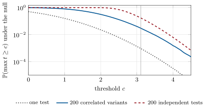
A research team tries two hundred variants of a momentum signal and presents the best: its backtest $t$ -statistic is 3.1, a one-sided $p$ -value of one in a thousand. Had none of the variants any edge, and had they been independent, the largest of two hundred $t$ -statistics would still exceed 3.1 with probability 17.6%, about one time in six. The variants are not independent, which helps; the team also chose the sample period, the universe and the cost model, which does not. This chapter is about what a test can say: size and power and the lemma that makes the likelihood ratio the right statistic; the many quiet choices that multiply the tests a researcher runs; the corrections that control the chance of any false discovery, or their proportion; and the tests built for the search over strategies, which respect the correlation between them.

12.1 Tests, size and power

Definition 12.1 (Hypothesis test, null hypothesis, $p$ -value)

A hypothesis test is a rule that, from data $X$ , decides whether to reject a null hypothesis $H_0$ (a statement about the law of $X$ , such as “the strategy’s mean return is zero”) in favour of an alternative $H_1$ . It rejects when a statistic $T(X)$ exceeds a critical value. The $p$ -value of an observed $t$ is $\P_{H_0}(T \ge t)$ : the probability, under the null, of a statistic at least as extreme as the one seen.

A $p$ -value is not the probability that the null is true, and one minus it is not the probability that the strategy works: both of those need a prior (chapter 14). It is a statement about the data under one hypothesis.

Definition 12.2 (Size, power)

The size of a test is the largest probability of rejecting when the null is true (a false positive, or type I error). The power of a test at an alternative is the probability of rejecting when that alternative is true; one minus the power is the type II error.

Theorem 12.3 (Neyman–Pearson lemma)

For a simple null (density $f_0$ ) against a simple alternative ( $f_1$ ), the test that rejects when $f_1(x)/f_0(x) > k$ , with $k$ chosen so that its size is $\alpha$ , is most powerful: no test of size at most $\alpha$ has higher power.

Proof. Let $\phi^*$ be the likelihood-ratio test and $\phi$ any test of size at most $\alpha$ (both indicator functions of the rejection region). Pointwise $(\phi^* - \phi)(f_1 - kf_0) \ge 0$ : where $\phi^* = 1$ , $f_1 > kf_0$ ; where $\phi^* = 0$ , $f_1 \le kf_0$ . Integrating, $\text{power}(\phi^*) - \text{power}(\phi) \ge k(\alpha - \text{size}(\phi)) \ge 0$ . ∎

For the mean of normal returns, the ratio $f_1/f_0$ against any positive mean is increasing in the sample mean, so the one-sided $t$ -test is the most powerful test of “no edge” against every positive edge at once. With composite hypotheses and nuisance parameters, the lemma becomes a recipe.

Definition 12.4 (Likelihood-ratio test)

The likelihood-ratio test of a null that imposes $r$ restrictions on $\theta$ rejects for large $\mathrm{LR} = 2\bigl(\ell(\hat\theta) - \ell(\hat\theta_0)\bigr)$ , where $\ell$ is the log-likelihood, $\hat\theta$ its maximiser and $\hat\theta_0$ its maximiser under the restrictions.

By Wilks’ theorem, under the null and regularity conditions (the true parameter inside the parameter space), $\mathrm{LR}$ is asymptotically $\chi^2_r$ . The condition matters in practice: testing that a Hawkes excitation (chapter 7) is zero puts the null on the boundary $\alpha = 0$ , and the limit becomes an equal mixture of a point mass at zero and a $\chi^2_1$ , which halves the $p$ -value.

Definition 12.5 (Kolmogorov–Smirnov test)

The Kolmogorov–Smirnov test of the null that $X_1, \dots, X_n$ are iid with a fully specified continuous cdf $F$ uses $D_n = \sup_x|F_n(x) - F(x)|$ , $F_n$ the empirical cdf. Under the null, $\P(\sqrt n\,D_n > \lambda) \to 2\sum_{k \ge 1}(-1)^{k-1}e^{-2k^2\lambda^2}$ , whatever $F$ ; the 5% critical value is $\lambda = 1.358$ .

A thousand daily returns drawn from a Student $t$ with four degrees of freedom, scaled to 1% volatility, give $D_n = 0.0615$ against the normal law with the same volatility: above the critical value $1.358/\sqrt{1\,000} = 0.0429$ , a $p$ -value of 0.0010. Two cautions come with the test. It is weakest in the tails, where $F_n - F$ is small even when the tails are wrong; and when the mean and variance are estimated from the same data, $D_n$ is smaller than the tabulated law assumes, so the critical values must be simulated for the fitted family (the Lilliefors correction).

The sharpest use of size and power in a research group is the question of how long to wait.

Proposition 12.6 (Sample size for a Sharpe ratio)

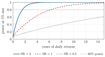
With $T$ years of independent returns and an annual Sharpe ratio $\mathrm{SR}$ , the one-sided test of $\mathrm{SR} = 0$ at size $\alpha$ has power approximately $\Phi\bigl(\mathrm{SR}\sqrt T - z_{1-\alpha}\bigr)$ , and reaches power $1 - \beta$ after

T = \Bigl(\frac{z_{1-\alpha} + z_{1-\beta}}{\mathrm{SR}}\Bigr)^2 \text{ years}.

Proof. By the delta method of chapter 11, the annualised estimate is approximately $\mathcal N(\mathrm{SR}, 1/T)$ when the daily ratio is small. The test rejects when $\widehat{\mathrm{SR}}\sqrt T > z_{1-\alpha}$ , which has probability $\Phi(\mathrm{SR}\sqrt T - z_{1-\alpha})$ ; setting it to $1 - \beta$ gives $T$ . ∎

At 5% size and 80% power, a Sharpe ratio of 2 needs 1.5 years, a Sharpe ratio of 1 needs 6.2 years and a Sharpe ratio of 0.5 needs 24.7 years (Figure 12.1). Five years of a genuine Sharpe ratio of 1 are detected 72% of the time: more than one in four good strategies fails its first honest test.

**Figure 12.1.** Power of the one-sided 5% test of a zero Sharpe ratio against years of independent daily returns, for true annual Sharpe ratios of 2, 1 and 0.5. The line at 80% power is crossed after 1.5, 6.2 and 24.7 years. Data: the chapter’s tutorial module.

12.2 The garden of forking paths

Definition 12.7 (Multiple testing, data snooping, garden of forking paths)

Multiple testing is running many tests and reporting some of them. Data snooping is choosing a model, a strategy or a parameter by searching over the same data that then test it, so that the reported statistic is the best of a search presented as a single test. The garden of forking paths is the implicit version: every choice the analyst would have made differently had the data been different (the sample period, the universe, the filter, the cost model) multiplies the tests actually run, even when only one analysis is ever performed.

The name is Gelman and Loken’s (2013), and the point is theirs: a researcher who never runs two backtests can still snoop, because the one backtest was shaped by looking at the data. A search is only corrected for if it is counted.

Proposition 12.8 (The maximum of independent statistics)

If $Z_1, \dots, Z_N$ are independent standard normal, $\P(\max_i Z_i \ge c) = 1 - \Phi(c)^N$ , and $\E[\max_i Z_i] \sim \sqrt{2\ln N}$ as $N \to \infty$ .

Proof. $\P(\max_i Z_i < c) = \prod_i\P(Z_i < c) = \Phi(c)^N$ . For the growth, $1 - \Phi(c) \approx \varphi(c)/c$ , and the maximum sits where $N(1 - \Phi(c)) \approx 1$ , that is $c^2/2 \approx \ln N$ to leading order. ∎

The asymptote is slow: for $N = 200$ the expected maximum is 2.75, not $\sqrt{2\ln200} = 3.26$ . That maximum of two hundred noise statistics clears the conventional $t > 2$ bar almost always, and the hook’s 3.1 about one time in six (Figure 12.2). A single test at $t = 3.1$ has $p = 0.001$ ; the best of two hundred independent tests at $t = 3.1$ has $p = 0.176$ .

Probability that the largest t-statistic reaches c when nothing works: one test, the two hundred momentum variants of the tutorial (Gaussian simulation with their estimated correlation), and two hundred independent tests. At the best variant’s 3.11 (vertical line): 0.0009, 0.030 and 0.17. Data: the chapter’s tutorial, seeded. — **Figure 12.2.** Probability that the largest $t$ -statistic reaches $c$ when nothing works: one test, the two hundred momentum variants of the tutorial (Gaussian simulation with their estimated correlation), and two hundred independent tests. At the best variant’s 3.11 (vertical line): 0.0009, 0.030 and 0.17. Data: the chapter’s tutorial, seeded.

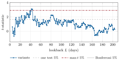
Real searches are correlated. The tutorial’s family is two hundred trend rules that hold the sign of the trailing $L$ -day return, for lookbacks $L = 5, \dots, 204$ days, applied to ten years of a driftless random walk with 1% daily volatility: no rule has any edge. Neighbouring lookbacks share almost all their signals (the best variant’s daily P&L has correlation 0.95 with its neighbour’s), distant ones much less (0.28 with the 5-day rule, 0.20 with the 204-day rule). In the history shown, 33 of the 200 variants have a one-sided $p$ -value below 5%, the mean $t$ -statistic across the family is 1.04 rather than zero, since every variant sees the same trending episodes, and the best, at a 42-day lookback, has $t = 3.11$ and an annualised Sharpe ratio of 0.98 (Figure 12.3). That history is the 336th we simulated: we drew histories until the best variant came near the hook’s 3.1, which is the chapter’s subject enacted on the chapter itself.

The t-statistics of the two hundred trend rules on one simulated ten-year random walk, against their lookback, with three one-sided 5% thresholds: a single test (1.645), the max-statistic critical value for this correlated family (2.92) and Bonferroni’s (3.48). The best rule, at 42 days, has t = 3.11. Data: the chapter’s tutorial, seeded. — **Figure 12.3.** The $t$ -statistics of the two hundred trend rules on one simulated ten-year random walk, against their lookback, with three one-sided 5% thresholds: a single test (1.645), the max-statistic critical value for this correlated family (2.92) and Bonferroni’s (3.48). The best rule, at 42 days, has $t = 3.11$ . Data: the chapter’s tutorial, seeded.

12.3 Family-wise error and false discoveries

Definition 12.9 (Family-wise error rate, Bonferroni correction, Holm procedure)

For $m$ hypotheses of which $m_0$ are true, the family-wise error rate (FWER) of a procedure is the probability that it rejects at least one true null. The Bonferroni correction rejects $H_i$ when $p_i \le \alpha/m$ . The Holm procedure orders the $p$ -values $p_{(1)} \le \dots \le p_{(m)}$ and rejects $H_{(1)}, \dots, H_{(k)}$ , where $k$ is the last index with $p_{(j)} \le \alpha/(m - j + 1)$ for every $j \le k$ .

Proposition 12.10 (Bonferroni and Holm control the family-wise error rate)

Under any dependence between the tests, both procedures have FWER at most $\alpha$ ; Holm rejects everything Bonferroni rejects.

Proof. Bonferroni: the union bound over the true nulls gives $\P(\exists i \in \mathcal H_0: p_i \le \alpha/m) \le m_0\alpha/m \le \alpha$ . Holm: let $j^*$ be the rank of the smallest $p$ -value among the true nulls. At most $m - m_0$ hypotheses precede it, so $j^* \le m - m_0 + 1$ , and Holm rejects a true null only if $p_{(j^*)} \le \alpha/(m - j^* + 1) \le \alpha/m_0$ , which by the union bound over the $m_0$ true nulls has probability at most $\alpha$ . Holm’s thresholds are never below $\alpha/m$ . ∎

Controlling the chance of any false discovery is the right goal when one false discovery is expensive, as when a single strategy goes live. When a research group screens hundreds of signals for a combined model, a few false ones among many true ones cost little, and demanding none throws away most of the true ones.

Definition 12.11 (False discovery rate, Benjamini–Hochberg procedure)

If a procedure makes $R$ rejections of which $V$ are true nulls, its false discovery rate is $\E[V/\max(R, 1)]$ . The Benjamini–Hochberg procedure at level $q$ rejects $H_{(1)}, \dots, H_{(k)}$ for the largest $k$ with $p_{(k)} \le kq/m$ .

Theorem 12.12 (Benjamini–Hochberg)

If the $p$ -values of the true nulls are independent of each other and of the others, the Benjamini–Hochberg procedure has false discovery rate exactly $q\,m_0/m \le q$ . It remains at most $q$ under positive regression dependence, and at most $q$ under any dependence if $q$ is replaced by $q/\sum_{k=1}^m k^{-1}$ (Benjamini and Yekutieli, 2001).

Example 12.13 (Five $p$ -values)

Take $p = (0.005, 0.01, 0.03, 0.04, 0.2)$ and $\alpha = q = 5\%$ . Bonferroni’s threshold $0.01$ rejects two. Holm compares them in order with $0.05/5, 0.05/4, 0.05/3, \dots$ : $0.005 \le 0.01$ and $0.01 \le 0.0125$ , then $0.03 > 0.0167$ stops it at two. Benjamini–Hochberg compares with $0.01, 0.02, 0.03, 0.04, 0.05$ : the largest $k$ with $p_{(k)} \le 0.01k$ is $k = 4$ , so it rejects four. As adjusted $p$ -values (the smallest level at which each is rejected): Bonferroni $(0.025, 0.05, 0.15, 0.2, 1)$ , Holm $(0.025, 0.04, 0.09, 0.09, 0.2)$ , Benjamini–Hochberg $(0.025, 0.025, 0.05, 0.05, 0.2)$ .

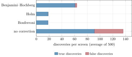
The trade shows at scale. Among a thousand candidate signals of which a hundred are real (with $t$ -statistics centred on 3), the naive 5% test makes 136 discoveries of which 45 are false; Bonferroni and Holm make about 18, with a false one in 5% of screens; Benjamini–Hochberg at 5% makes 63, of which 2.9 are false on average, a false discovery rate of 4.4% against the theorem’s $0.05 \times 900/1\,000 = 4.5\%$ (Figure 12.4). It pays for its power with a family-wise error rate of 92%: almost every screen contains a false signal, and that is the design.

**Figure 12.4.** A thousand signals, a hundred of them real: average true and false discoveries of four rules at 5%. No correction: 91 true, 45 false. Bonferroni and Holm: 18 true, 0.05 false. Benjamini–Hochberg: 61 true, 2.9 false (a false discovery rate of 4.4%). Data: the chapter’s tutorial, seeded.

On the momentum family neither control is kind. Bonferroni and Holm both give the best variant an adjusted $p$ -value of $200 \times 0.00094 = 0.187$ ; Benjamini–Hochberg gives 0.076, smaller because its step-up borrows strength from the 33 other small $p$ -values. No variant survives either at 5%. But both corrections were built for the worst case of dependence, and two hundred variants that share most of their signals are far from two hundred independent chances.

12.4 Reality-check tests for strategy search

Definition 12.14 (Reality Check, superior predictive ability test)

For $K$ strategies with performance series $d_{k,t}$ in excess of a benchmark, the Reality Check (White, 2000) tests $H_0: \max_k\E[d_k] \le 0$ with the statistic $\max_k\sqrt n\,\bar d_k$ , whose null distribution is estimated by the bootstrap of $\max_k\sqrt n(\bar d_k^* - \bar d_k)$ . The superior predictive ability test (Hansen, 2005) studentises each $\bar d_k$ and recentres only the strategies that are not clearly worse than the benchmark, so that adding poor strategies to the search does not make the test more conservative.

Both tests replace the union bound by the actual law of the maximum, and the bootstrap (chapter 13) keeps the dependence between strategies and over time. When the statistics are approximately jointly normal, a Gaussian simulation with their estimated correlation does the same job at no cost.

Method 12.15 (Max-statistic $p$ -values)

Given $t$ -statistics $t_1, \dots, t_m$ and the correlation matrix $R$ of the underlying P&L series: draw $Z^{(s)} \sim \mathcal N(0, R)$ for $s = 1, \dots, S$ ; the adjusted $p$ -value of $H_i$ is the share of draws with $\max_j Z_j^{(s)} \ge t_i$ . The step-down version (Romano and Wolf, 2005) takes the maximum, for the $k$ -th largest statistic, only over the hypotheses not yet rejected. Both control the family-wise error rate; the effective number of independent trials of the search is the $N$ that solves $1 - (1 - p_{\text{naive}})^N = p_{\text{adjusted}}$ .

For the momentum family, 200 000 draws from the estimated correlation give the best variant an adjusted $p$ -value of 0.030, against 0.187 for Bonferroni and 0.171 for two hundred independent tests. The search over two hundred correlated lookbacks amounts to 32 independent trials. The max-statistic 5% critical value is 2.92, well below Bonferroni’s 3.48, and three variants clear it. The check that matters: over 2 000 fresh ten-year histories, the best variant reaches $t = 3.11$ in 2.6% of them, close to the simulated 3.0%.

So the corrected test rejects, at 5%, a strategy that has no edge. It is allowed to, 3% of the time; and this history was the 336th we drew. The correction accounts for the two hundred lookbacks it was told about and for nothing else: not the histories we discarded, not the other signal families the team tried last year. Harvey, Liu and Zhu (2016) reach a similar conclusion for published equity factors, arguing that a new factor should clear a $t$ -statistic of about 3 rather than 2.

Definition 12.16 (Deflated Sharpe ratio)

For a Sharpe ratio $\widehat{\mathrm{SR}}$ (per period) estimated from $n$ returns with skewness $\gamma_3$ and kurtosis $\gamma_4$ , the probability that the true ratio exceeds $\mathrm{SR}_0$ is approximately

\Phi\Bigl((\widehat{\mathrm{SR}} - \mathrm{SR}_0)\sqrt{n - 1}\Big/\sqrt{1 - \gamma_3\widehat{\mathrm{SR}} + \tfrac{\gamma_4 - 1}4\widehat{\mathrm{SR}}^2}\Bigr).

The deflated Sharpe ratio (Bailey and López de Prado, 2014) is this probability with $\mathrm{SR}_0$ the expected maximum of $N$ null Sharpe ratios of variance $V$ : $\mathrm{SR}_0 = \sqrt V\bigl((1 - \gamma_E)\Phi^{-1}(1 - 1/N) + \gamma_E\Phi^{-1}(1 - 1/(Ne))\bigr)$ , $\gamma_E$ the Euler–Mascheroni constant.

For the best momentum variant the probability that its true Sharpe ratio is positive is 0.999, the single-test view. Deflated for two hundred trials (with $V = 1/n$ , the null variance), the benchmark becomes an annual 0.87 and the deflated Sharpe ratio 0.63; for the 32 effective trials, 0.67 and 0.84. Neither reaches the 0.95 a desk would want, and the number of trials, which the researcher controls and the reader rarely sees, moves the answer more than the data do.

12.5 Tutorial: the best of two hundred

Goal. Search two hundred worthless trend rules, pick the best, and measure how surprising it is under five corrections. End state: Figures 12.3 and 12.2 and the adjusted $p$ -values 0.187, 0.076 and 0.030.

Adjusted $p$ -values by Holm’s step-down and Benjamini–Hochberg’s step-up.

def holm(p) -> np.ndarray:
    """Step-down: the k-th smallest p-value (k = 1..m) is multiplied by m - k + 1, then made monotone."""
    p = _check(p)
    m = p.size
    order = np.argsort(p)
    adj = np.maximum.accumulate((m - np.arange(m)) * p[order])
    out = np.empty(m)
    out[order] = np.minimum(1.0, adj)
    return out


def benjamini_hochberg(p, dependence_factor: float = 1.0) -> np.ndarray:
    """Step-up: the k-th smallest p-value is multiplied by m / k, then made monotone from the top."""
    p = _check(p)
    m = p.size
    order = np.argsort(p)
    ranked = p[order] * m * dependence_factor / np.arange(1, m + 1)
    adj = np.minimum.accumulate(ranked[::-1])[::-1]
    out = np.empty(m)
    out[order] = np.minimum(1.0, adj)
    return out

Listing 12.1. Holm and Benjamini–Hochberg adjusted

p

-values. code/firm/multitest/firm_multitest.py

Max-statistic $p$ -values from a Gaussian null with the estimated correlation, or from any matrix of null draws.

def _gaussian_null(corr: np.ndarray, n_sim: int, seed: int) -> np.ndarray:
    w, v = np.linalg.eigh(0.5 * (corr + corr.T))
    root = v * np.sqrt(np.clip(w, 0.0, None))
    rng = np.random.default_rng(seed)
    out = np.empty((n_sim, corr.shape[0]))
    for a in range(0, n_sim, 10_000):                      # blocks keep memory flat
        b = min(n_sim, a + 10_000)
        out[a:b] = rng.standard_normal((b - a, corr.shape[0])) @ root.T
    return out


def maxt_pvalues(t, corr=None, n_sim: int = 100_000, seed: int = 0, null_draws=None,
                 stepdown: bool = False) -> np.ndarray:
    """One-sided max-statistic adjusted p-values: P(max_j Z_j >= t_i) under the joint null.

    The null is Gaussian with correlation `corr` (identity if None), or the rows of `null_draws`
    (n_sim x m, e.g. bootstrap statistics centred on the null). With stepdown=True the maximum for the
    k-th largest statistic runs over the hypotheses not yet rejected (Romano-Wolf), which is uniformly
    less conservative and still controls the family-wise error rate.
    """
    t = np.asarray(t, dtype=float)
    m = t.size
    if null_draws is None:
        null_draws = _gaussian_null(np.eye(m) if corr is None else np.asarray(corr, float), n_sim, seed)
    null_draws = np.asarray(null_draws, dtype=float)
    if not stepdown:
        mx = np.sort(null_draws.max(axis=1))
        return 1.0 - np.searchsorted(mx, t, side="left") / mx.size
    order = np.argsort(-t)
    adj = np.empty(m)
    for k, i in enumerate(order):
        mx = null_draws[:, order[k:]].max(axis=1)
        adj[k] = np.mean(mx >= t[i])
    adj = np.maximum.accumulate(adj)
    out = np.empty(m)
    out[order] = adj
    return out

Listing 12.2. Single-step and step-down max-statistic

p

-values. code/firm/multitest/firm_multitest.py

Run problem() in qm_testing.py, then family_exceedance(3.11) to check the simulated $p$ -value on fresh histories, and fig_testing.py.

What to change next. Add the mirror-image reversal rules and see the effective number of trials grow; replace the Gaussian null by the stationary bootstrap of chapter 13 through the null_draws hook.

12.6 Build: the multiple-testing module

Purpose. Every strategy the miniature firm promotes from research carries the size of the search behind it and an adjusted $p$ -value; this module computes them.

Interface. bonferroni(p), holm(p), benjamini_hochberg(p), benjamini_yekutieli(p) returning adjusted $p$ -values; maxt_pvalues(t, corr, n_sim, seed, null_draws, stepdown); effective_trials(p_single, p_family); expected_max_sr(n_trials, sr_var); deflated_sharpe(sr, n_obs, skew, kurt, sr0); norm_cdf, norm_ppf.

Rules. Adjusted $p$ -values, not reject flags, so that the level is chosen by the caller; one-sided statistics for strategy search; the null draws are a parameter, so that the bootstrap replaces the Gaussian without touching the callers.

Acceptance tests. code/firm/multitest/tests/: the five- $p$ -value example; FWER and FDR control by simulation; the max-statistic $p$ -value equals the independent formula for $R = I$ and the naive $p$ -value for perfectly correlated tests; the expected-maximum approximation within 1.5%.

Stretch. Hansen’s SPA test with the stationary bootstrap; the Romano–Wolf step-down with bootstrap null draws; the probability of backtest overfitting by combinatorial cross-validation.

Sources and further reading

J. Neyman and E. S. Pearson, “On the problem of the most efficient tests of statistical hypotheses”, Philosophical Transactions of the Royal Society A 231, 1933.
S. Holm, “A simple sequentially rejective multiple test procedure”, Scandinavian Journal of Statistics 6, 1979.
Y. Benjamini and Y. Hochberg, “Controlling the false discovery rate: a practical and powerful approach to multiple testing”, Journal of the Royal Statistical Society B 57, 1995.
Y. Benjamini and D. Yekutieli, “The control of the false discovery rate in multiple testing under dependency”, Annals of Statistics 29, 2001.
H. White, “A reality check for data snooping”, Econometrica 68, 2000.
P. R. Hansen, “A test for superior predictive ability”, Journal of Business and Economic Statistics 23, 2005.
J. P. Romano and M. Wolf, “Stepwise multiple testing as formalized data snooping”, Econometrica 73, 2005.
C. R. Harvey, Y. Liu and H. Zhu, “…and the cross-section of expected returns”, Review of Financial Studies 29, 2016.
D. H. Bailey and M. López de Prado, “The deflated Sharpe ratio”, Journal of Portfolio Management 40(5), 2014.
A. Gelman and E. Loken, “The garden of forking paths”, working paper, 2013.

12.7 Exercises

Exercise 12.1 ★

A backtest has $t = 2.5$ . What is its one-sided $p$ -value, and its Bonferroni-adjusted $p$ -value if it is the best of twenty variants?

Solution

Solution of Exercise 12.1.

$p = 1 - \Phi(2.5) = 0.0062$ ; Bonferroni over twenty variants, $20 \times 0.0062 = 0.124$ : not significant at 5%.

Exercise 12.2 ★

A test rejects when $Z > 1.645$ . Under the alternative of interest $Z \sim \mathcal N(2, 1)$ . What are its size and its power?

Solution

Solution of Exercise 12.2.

Size $1 - \Phi(1.645) = 5\%$ ; power $\P(\mathcal N(2, 1) > 1.645) = \Phi(0.355) = 0.639$ .

Exercise 12.3 ★

Apply Bonferroni and Holm at 5% to $p = (0.001, 0.012, 0.02, 0.3)$ .

Solution

Solution of Exercise 12.3.

Bonferroni’s threshold is 0.0125: it rejects the first two. Holm compares the ordered $p$ -values with 0.0125, 0.0167, 0.025 and 0.05 in turn: 0.001, 0.012 and 0.02 pass and 0.3 does not, so it makes three rejections. The adjusted $p$ -values are, for Bonferroni, 0.004, 0.048, 0.08 and 1; for Holm, 0.004, 0.036, 0.04 and 0.3.

Exercise 12.4 ★★

How many years of independent returns does a test of 5% size need to detect an annual Sharpe ratio of 0.7 with 90% power?

Solution

Solution of Exercise 12.4.

$T = ((1.645 + 1.282)/0.7)^2 = 17.5$ years.

Exercise 12.5 ★★

Daily returns are normal with mean zero. The first 500 days have sample variance $(1.0\%)^2$ , the next 500 $(1.2\%)^2$ . Compute the likelihood-ratio statistic for a common variance and its $p$ -value.

Solution

Solution of Exercise 12.5.

With known zero mean, $\mathrm{LR} = n\ln\hat s^2 - n_1\ln\hat s_1^2 - n_2\ln\hat s_2^2$ with the pooled $\hat s^2 = (1 + 1.44)/2 = 1.22$ (in $\%^2$ ): $1\,000\ln1.22 - 500\ln1.44 = 16.53$ . Against $\chi^2_1$ , $p = 4.8 \times 10^{-5}$ : the variance changed.

Exercise 12.6 ★★

For ten independent noise strategies, what is the probability that the best has $t \ge 2$ , and what is the expected maximum by the formula of the deflated Sharpe ratio?

Solution

Solution of Exercise 12.6.

$1 - \Phi(2)^{10} = 1 - 0.97725^{10} = 0.206$ . The formula gives $(1 - \gamma_E)\Phi^{-1}(0.9) + \gamma_E\Phi^{-1}(1 - 1/(10e)) = 1.57$ (the exact expected maximum is 1.54).

Exercise 12.7 ★★★

Coding. Repeat the thousand-signal screen with null statistics that share a common factor (correlation 0.5). Does Benjamini–Hochberg still control the false discovery rate at 5%? How often does the realised proportion of false discoveries exceed 10%?

Solution

Solution of Exercise 12.7.

With 500 screens (fdr_correlated()): the false discovery rate is 3.0%, within the 5% bound (positive dependence), with about 63 discoveries per screen. But the realised proportion is volatile: it exceeds 10% in 7.8% of screens, when the common factor pushes all the null statistics up together. The procedure controls an average, not each screen.

Exercise 12.8 ★★★

Find the flaw. “We tested our signal separately on twelve markets. It is significant at 5% in three of them, where we now trade it; the three backtests are our estimate of its performance.”

Solution

Solution of Exercise 12.8.

Twelve tests at 5% produce 0.6 false positives on average; three or more occur with probability 2.0% if the signal is useless everywhere and the markets independent, so the count is mild evidence of something. The flaw is the selection: the three winners were chosen because their backtests were good, so their in-sample performance is biased upward (the winner’s curse), and the markets are not independent. Report the family result, and estimate performance on data not used to choose the markets.

12.8 Problem: Two Hundred Momentum Variants

Problem 12.1

Weekend problem — how surprising is the best of a correlated search?

A team backtests two hundred trend rules (hold the sign of the trailing $L$ -day return, $L = 5, \dots, 204$ ) on ten years of a market that, unknown to them, is a driftless random walk with 1% daily volatility. The history is the chapter’s seeded one.

Part I — The search.

Which lookback wins, with what $t$ -statistic and annualised Sharpe ratio?
What is its naive one-sided $p$ -value?
How many of the two hundred pass a one-sided 5% test?
What is the mean $t$ -statistic across the family, and why is it not near zero?
What is the correlation of the best rule’s P&L with its neighbour’s, and with the 5-day and 204-day rules’?

Part II — Corrections.

What are the Bonferroni-adjusted $p$ -value and the Bonferroni critical value?
What does Holm give for the best, and why the same?
What does Benjamini–Hochberg give, and why smaller?
What would the adjusted $p$ -value be if the two hundred were independent?
What are the max-statistic adjusted $p$ -value and critical value, from the estimated correlation?

Part III — What the search amounts to.

What is the effective number of independent trials?
How many variants clear the max-statistic threshold?
Over 2 000 fresh histories, how often does the best rule reach $t = 3.11$ ?
What are the probabilistic Sharpe ratio and the deflated Sharpe ratio with 200 and with the effective number of trials?
Do the answers change if daily returns have Student- $t$ tails with four degrees of freedom?

Part IV — Judgement.

The rules have no edge by construction. Why does the corrected test reject?
What would you require before trading the 42-day rule?
What should the research report record about the search?
State the named result: the adjusted $p$ -value of the best of two hundred correlated variants and the effective number of trials.
In one sentence: what does a multiple-testing correction protect against, and what not?

Solution

Solution of Problem 12.1.

1. Lookback 42 days: $t = 3.11$ , annualised Sharpe ratio 0.98. 2. $p = 1 - \Phi(3.11) = 0.00094$ . 3. 33 of 200. 4. 1.04: every rule trades the same history, so its trending episodes lift the whole family together. 5. 0.95 with the 43-day rule; 0.28 with the 5-day and 0.20 with the 204-day rule. 6. $200 \times 0.00094 = 0.187$ ; critical value $\Phi^{-1}(1 - 0.05/200) = 3.48$ . 7. 0.187: Holm multiplies the smallest $p$ -value by $m$ , as Bonferroni does; it gains only further down the list. 8. 0.076: the step-up takes the minimum of $p_{(k)}m/k$ over the ranks above, and the 33 small $p$ -values make those small. 9. $1 - (1 - 0.00094)^{200} = 0.171$ . 10. 0.030 from 200 000 Gaussian draws with the estimated correlation; the 5% critical value of the maximum is 2.92. 11. $\ln(1 - 0.030)/\ln(1 - 0.00094) = 32$ trials. 12. Three. 13. In 2.6% of them, close to the simulated 3.0% (the sampling error of 2 000 histories is 0.4 points). 14. The probability that the true Sharpe ratio is positive is 0.999. Deflated for 200 trials: benchmark 0.87 a year, deflated Sharpe ratio 0.63; for 32 trials: 0.67 and 0.84. 15. Barely: with Student- $t_4$ returns the best rule reaches 3.11 in 2.35% of 2 000 fresh histories; the $t$ -statistics are still close to normal after 2 520 days. 16. A 5% test rejects a true null 5% of the time, and the best rule’s adjusted $p$ -value is 3%; besides, the history is the 336th drawn, a search the correction was not told about. 17. A holdout never used in the search, an economic reason for trend at that horizon, performance net of costs, and an adjusted $p$ -value that counts every family the team tried. 18. The number of variants and families tried, their correlation, the adjusted $p$ -values and the method, the sample period and what was fixed before looking at the data. 19. Named result: the best of two hundred: the best of two hundred correlated momentum rules, naive $p = 0.00094$ , has a max-statistic adjusted $p$ -value of 0.030 (Bonferroni: 0.187); the search amounts to 32 independent trials. 20. It protects against the searches it is told about, and against nothing the researcher did not count.

12.9 Interview questions

Interview question 12.1 ★ researcher, trader

What is a $p$ -value, and what is it not?

Solution

Solution of Interview question 12.1.

The probability, if the null is true, of a statistic at least as extreme as the one observed. It is not the probability that the null is true, not the probability that the result will repeat, and not a measure of the size of the effect.

What the interviewer is looking for: The conditional direction ( $\P(\text{data} \mid H_0)$ , not $\P(H_0 \mid \text{data})$ ), and that effect size needs its own number.

Interview question 12.2 ★★ researcher, trader

You backtested a hundred strategies and the best has $t = 2.8$ . Is it real?

Solution

Solution of Interview question 12.2.

Probably not. If all were noise and independent, the best of 100 exceeds 2.8 with probability $1 - \Phi(2.8)^{100} = 0.23$ ; correlation lowers that, but then ask how many variants and choices came before the hundred. Adjust for the search (max-statistic or Bonferroni), then test on a holdout.

What the interviewer is looking for: The one-in-four arithmetic, the effect of correlation, and a holdout as the real test.

Interview question 12.3 ★★ researcher, mle

Bonferroni or Benjamini–Hochberg: when would you use which?

Solution

Solution of Interview question 12.3.

Bonferroni or Holm (family-wise error) when one false positive is costly, such as the one strategy that goes live; Benjamini–Hochberg (false discovery rate) when screening many candidates for a combined model, where a few false ones among many true ones are acceptable. Under strong dependence use the max-statistic version or Benjamini–Yekutieli.

What the interviewer is looking for: Matching the error rate to the cost of a false discovery; Holm dominates Bonferroni.

Interview question 12.4 ★★ researcher, trader, risk

How long must a strategy run before you can confirm a Sharpe ratio of 1?

Solution

Solution of Interview question 12.4.

The annual estimate has standard error about $1/\sqrt T$ , so $t = \sqrt T$ : four years for $t = 2$ , and at 5% size with 80% power $(1.645 + 0.842)^2 = 6.2$ years. Autocorrelated returns and fat tails make it longer; a search makes it longer still.

What the interviewer is looking for: The $1/\sqrt T$ rule and the power calculation, not only $t = 2$ .

Interview question 12.5 ★★★ researcher

Your two hundred variants are highly correlated. How do you correct for the search?

Solution

Solution of Interview question 12.5.

Use the law of the maximum rather than the union bound: estimate the correlation of the variants’ P&L and simulate the maximum of correlated normals, or bootstrap the maximum jointly (Reality Check, SPA, Romano–Wolf step-down). Report the effective number of trials. Bonferroni is valid but very conservative here.

What the interviewer is looking for: Max-statistic over union bound, joint resampling that keeps the dependence, and counting families as well as variants.

Interview question 12.6 ★★ mle, researcher

What is the garden of forking paths, and where does it hide in a machine-learning pipeline?

Solution

Solution of Interview question 12.6.

The implicit multiplicity of choices that depend on the data even when one analysis is run. In machine learning: feature choices made after looking at validation scores, early stopping and hyperparameters tuned on the test set, reruns with new seeds until the curve looks good, and a test set reused across many model iterations until it becomes a training set.

What the interviewer is looking for: Concrete leak points, and the discipline of a holdout touched once.

Interview question 12.7 ★★ researcher, risk

You fit a distribution to returns and a Kolmogorov–Smirnov test does not reject it. What have you learned?

Solution

Solution of Interview question 12.7.

Little. The test is weak in the tails, which is where return distributions differ; with parameters fitted to the same data its tabulated critical values are too lenient (Lilliefors), so it rejects even less often; and failing to reject is not acceptance. Compare tail quantiles or exceedance counts directly, with simulated critical values.

What the interviewer is looking for: Weak tail power, the fitted-parameter correction, and absence of evidence versus evidence of fit.

Terms defined in this chapter

See all 2333 terms in the glossary