Quantitative Methods · Methods

29Games, Auctions and Information

In November 1998 the United States Treasury moved every auction of marketable securities to a single clearing price: all winners pay the highest accepted yield, instead of each paying its own bid. It had run an experiment with two- and five-year notes since September 1992, and its own study of the experiment found that dealers bid more aggressively under the single price, that awards were less concentrated, and that the auction’s yield spread over the when-issued market roughly halved for two-year notes (from 0.41 to 0.22 of a basis point), a difference that was not statistically significant because results were more volatile from auction to auction. A dealer bids differently in the two formats. The theory of games and auctions says how, and whether the Treasury should have expected to raise more. This chapter develops that theory, and ends with the information theory of a bettor who buys a tip.

29.1 Games and equilibrium

Definition 29.1 (Normal-form game, Nash equilibrium, mixed strategy, zero-sum game)

A normal-form game is a set of players, a set of strategies for each and a payoff to each player for every profile of strategies. A mixed strategy is a probability distribution over a player’s strategies. A Nash equilibrium is a profile of (mixed) strategies in which no player gains by deviating alone. A zero-sum game is a two-player game whose payoffs sum to zero; with a payoff matrix $A$ for the row player, mixed strategies $x$ and $y$ give her $x^\top Ay$ .

Theorem 29.2 (Existence of equilibria; minimax)

Every finite game has a Nash equilibrium in mixed strategies (Nash, 1950; stated). In a finite zero-sum game, $\max_x\min_yx^\top Ay = \min_y\max_xx^\top Ay$ (von Neumann, 1928); the common value is the value of the game, and the optimal strategies form the equilibria.

Idea. Existence follows from Kakutani’s fixed-point theorem applied to the best-response correspondence. For the minimax theorem, the row player’s problem $\max\{v : A^\top x \ge v\mathbf 1, \mathbf 1^\top x = 1, x \ge 0\}$ is a linear programme whose dual is the column player’s problem, and strong duality (chapter 23) equates their values. ∎

In weighted rock–paper–scissors (rock beats scissors for 1, scissors beat paper for 1, paper beats rock for 2), the equilibrium is not uniform: each player plays rock, paper and scissors with probabilities $(\frac14, \frac12, \frac14)$ , and the value is zero. Two players who each run multiplicative weights for 20 000 rounds, reinforcing the actions that would have paid, average to $(0.250, 0.502, 0.248)$ with a duality gap of 0.005: the learning dynamics find the equilibrium neither player computed. Nash equilibria of non-zero-sum games are harder to compute and need not be unique; a trading desk meets them in quoting games (Book 2) and in the auctions below.

29.2 Bayesian games

Definition 29.3 (Bayesian game, Bayes–Nash equilibrium)

A Bayesian game (Harsanyi, 1967–68) adds to a game a type for each player, drawn from a common prior and known only to its owner; a strategy maps types to actions. A Bayes–Nash equilibrium is a strategy profile in which each type’s action maximises its expected payoff given its beliefs about the others’ types and their strategies.

Definition 29.4 (Private and common values, first- and second-price auctions)

In a private-value auction each bidder knows its own value for the object; in a common-value auction the value is the same for all and each bidder sees only a signal of it. In a first-price auction sealed bids are opened and the highest bidder pays its bid; in a second-price auction (Vickrey, 1961) the highest bidder pays the second-highest bid. Bid shading is bidding below one’s value.

Proposition 29.5 (Equilibrium bids)

With $n$ bidders whose values are independent with distribution function $F$ on $[0, 1]$ : in the second-price auction, bidding one’s value is weakly dominant; in the first-price auction, the symmetric Bayes–Nash equilibrium is $b(v) = v - \int_0^vF(x)^{n-1}dx/F(v)^{n-1}$ , which for uniform values is $b(v) = \frac{n-1}nv$ .

Proof. Second price: bidding $b \ne v$ changes the outcome only when the highest rival bid $h$ lies between $b$ and $v$ ; if $b > h > v$ the bidder wins and pays $h > v$ , a loss, and if $v > h > b$ it forgoes the profit $v - h$ . First price: if rivals use an increasing $b$ , a bidder with value $v$ who bids $b(w)$ wins with probability $F(w)^{n-1}$ and earns $(v - b(w))F(w)^{n-1}$ . The first-order condition at $w = v$ is $\frac{d}{dv}(b(v)F(v)^{n-1}) = v\frac{d}{dv}F(v)^{n-1}$ , and integrating by parts from $b(0) = 0$ gives the formula. ∎

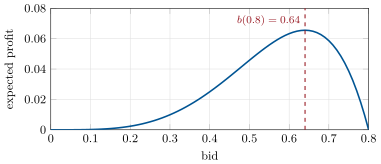
With five bidders and uniform values each shades its bid by exactly one fifth. The equilibrium is a best response bidder by bidder: a bidder with value 0.8 facing four rivals who bid $\frac45$ of their values maximises its expected profit at a bid of 0.64 (Figure 29.1). The shading is the price of not paying the second-highest bid: it recovers exactly the expected gap between one’s own value and the next one below.

Expected profit (v - b)\, ( win) of a bidder with value 0.8 in a first-price auction against four rivals with uniform values who bid 4/5 of their values: the best response is the equilibrium bid. Data: the chapter’s tutorial. — **Figure 29.1.** Expected profit $(v - b)\,\P(\text{win})$ of a bidder with value 0.8 in a first-price auction against four rivals with uniform values who bid $\frac45$ of their values: the best response is the equilibrium bid. Data: the chapter’s tutorial.

29.3 Auction formats and revenue

Definition 29.6 (English and Dutch auctions, reserve price)

An English auction raises the price until one bidder remains, who pays the price at which the last rival dropped out. A Dutch auction lowers the price until a bidder accepts it. A reserve price is the lowest price at which the seller will sell.

The English auction is strategically a second-price auction with private values (stay in until the price reaches your value), and the Dutch auction is a first-price auction (choose the price at which to stop).

Theorem 29.7 (Revenue equivalence)

With independent private values drawn from a common continuous distribution and risk-neutral bidders, every auction in which the highest value wins in equilibrium and a bidder with the lowest possible value expects zero surplus yields the same expected revenue (Vickrey, 1961; Myerson, 1981; Riley and Samuelson, 1981).

Idea. In any such equilibrium, a bidder’s expected surplus $U(v)$ satisfies the envelope condition $U'(v) = \P(\text{win} \mid v) = F(v)^{n-1}$ , so $U(v) = U(0) + \int_0^vF^{n-1}$ is fixed by the allocation rule. Its expected payment, $vF(v)^{n-1} - U(v)$ , is then the same in every format, and so is the seller’s revenue, the sum of the expected payments. ∎

With five bidders and uniform values, the expected revenue of every format is $\frac{n-1}{n+1} = \frac23$ . A million simulated auctions of each give 0.6665 (first price), 0.6665 (second price), 0.6715 for an English clock that rises by ticks of 0.01 and 0.6614 for a Dutch clock that falls by ticks of 0.01, the last two off by half a tick in opposite directions. The first-price winner pays its shaded bid, the second-price winner the second value; the averages agree, the distributions do not.

Proposition 29.8 (Optimal reserve price)

For regular value distributions, the revenue-maximising auction sets a reserve $r^*$ solving $r - (1 - F(r))/f(r) = v_0$ , the seller’s own value, independent of the number of bidders (Myerson, 1981; stated). For uniform values and $v_0 = 0$ , $r^* = \frac12$ , and with $n$ bidders the expected revenue is $\frac{n-1}{n+1} - \frac{2n}{n+1}r^{n+1} + r^n$ .

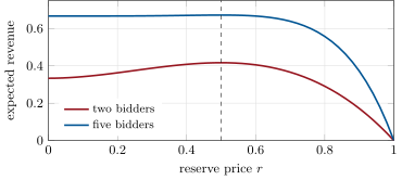
A reserve raises revenue by sometimes not selling. With two bidders the optimal reserve of 0.5 raises the expected revenue from $\frac13$ to $\frac5{12}$ , by 25%, and leaves the object unsold a quarter of the time; with five bidders it raises it from 0.6667 to 0.6719, by 0.8%, and leaves it unsold 3.1% of the time (Figure 29.2): competition does the reserve’s work.

Expected revenue of a standard auction with uniform private values against the reserve price; both curves peak at r* = 1/2. Data: the chapter’s tutorial (closed form, checked by simulation). — **Figure 29.2.** Expected revenue of a standard auction with uniform private values against the reserve price; both curves peak at $r^* = \frac12$ . Data: the chapter’s tutorial (closed form, checked by simulation).

Definition 29.9 (Pay-as-bid and discriminatory auctions)

A pay-as-bid auction, or discriminatory auction, sells several units to the highest bids, each winner paying its own bid; it is the multi-unit first-price auction, as the uniform-price auction of Book 2 is the multi-unit second-price auction.

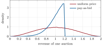
The Treasury’s switch can now be modelled. Take five dealers, each wanting one of two units, with uniform private values. In the uniform-price auction each bids its value, and revenue is twice the third-highest value, $2 \times \frac36 = 1$ in expectation. In the pay-as-bid auction a dealer with value $v$ bids the expected value of the second-highest of the other four given that it is below $v$ , $b(v) = v(3 - 2.4v)/(4 - 3v)$ : 0.36 at a value of 0.5, 0.54 at 0.8, 0.60 at 1. By revenue equivalence expected revenue is again 1; 400 000 simulated auctions give 0.9994 and 0.9999. What differs is everything else: under the uniform price the bids are spread twice as widely (the gap between the two winning bids averages 0.167 against 0.087) and the revenue varies more than twice as much from auction to auction (standard deviation 0.378 against 0.160; Figure 29.3), the two features the Treasury’s study reported. With unit demand the model cannot favour either format on average; real dealers demand many units and can shade their bids in a uniform-price auction too (demand reduction), which is why the question was empirical.

**Figure 29.3.** Distribution of revenue in 400 000 simulated auctions of two units to five unit-demand bidders with uniform private values, under the uniform-price and pay-as-bid formats in equilibrium: the same mean, 1, and very different spreads. Data: the chapter’s tutorial.

Common values change the logic. If the value $V$ is common and each of five bidders sees $V$ plus uniform noise on $\pm0.1$ , the highest signal overstates $V$ by $0.1 \times \frac46 = 0.067$ on average, and a bidder who bids its signal in a first-price auction loses that much when it wins, in 97% of its wins: the winner’s curse of Book 2. Shading by the expected overstatement brings the winners’ profit to zero. With affiliated values the formats no longer raise the same revenue: the English auction, which reveals the dropouts’ information, raises at least as much as the second-price auction, which raises at least as much as the first-price auction (Milgrom and Weber, 1982).

29.4 Entropy and optimal betting

Definition 29.10 (Entropy, mutual information)

The entropy of a discrete random variable $X$ is $H(X) = -\sum_xp(x)\log_2p(x)$ bits (Shannon, 1948). The mutual information of $X$ and $Y$ is $I(X; Y) = \sum_{x,y}p(x, y)\log_2\frac{p(x, y)}{p(x)p(y)} = H(X) - H(X \mid Y)$ , the Kullback–Leibler divergence of the joint law from the product of its marginals.

Theorem 29.11 (Kelly: the value of side information)

In a horse race with win probabilities $p(x)$ and decimal odds $o(x)$ , a bettor who stakes its whole wealth in proportions $b(x)$ has doubling rate $W(b) = \sum_xp(x)\log_2(b(x)o(x))$ , maximised by $b = p$ (the Kelly criterion of Book 2). With a signal $Y$ observed before each race, the optimal doubling rate rises by exactly $I(X; Y)$ bits per race, whatever the odds (Kelly, 1956).

Proof. $W(b) - W(p) = \sum_xp(x)\log_2(b(x)/p(x)) = -D(p\,\|\,b) \le 0$ , so $b = p$ is optimal and $W^* = \sum_xp(x)\log_2(p(x)o(x))$ . With the signal, the optimal stakes are $p(x \mid y)$ and

W^*_Y = \sum_{x,y}p(x, y)\log_2(p(x \mid y)o(x)).

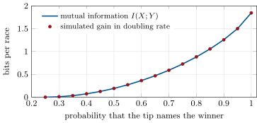
The odds cancel in the difference: $W^*_Y - W^* = \sum_{x,y}p(x, y)\log_2\frac{p(x \mid y)}{p(x)} = I(X; Y)$ . ∎

A four-horse race with probabilities $(0.4, 0.3, 0.2, 0.1)$ and decimal odds $(2.2, 3, 4.5, 9)$ , where the track keeps about 11% (the implied probabilities sum to 1.12), has entropy 1.846 bits. The best bettor loses 0.165 bits a race: its wealth halves every six races or so. A tip that names the winner with probability 0.6 (and one of the others at random otherwise) carries 0.363 bits, and turns the doubling rate to $+0.198$ ; 200 000 simulated races give a gain of $0.363 \pm 0.002$ . A tip right with probability $\frac14$ carries nothing, and a perfect tip carries the whole entropy (Figure 29.4). Information has a price in bits, and the bits are exactly the growth.

**Figure 29.4.** Gain in the Kelly bettor’s doubling rate from a noisy tip, against the tip’s accuracy, in a four-horse race: the mutual information and the gain measured over 200 000 simulated races for each accuracy. Data: the chapter’s tutorial, seeded.

29.5 Tutorial: the Treasury’s switch

Goal. Check revenue equivalence in four single-unit formats and two multi-unit formats, price a reserve, show the winner’s curse, and measure the value of a tip in bits. End state: the figures and the named numbers of the weekend problem.

Equilibrium bids. First-price (closed form and general), and pay-as-bid with unit demand.

def fp_bid(v, n: int, reserve: float = 0.0):
    """b(v) = v - (v^n - r^n) / (n v^(n-1)) for v >= r (uniform values); bidders below the reserve do not bid."""
    v = np.asarray(v, dtype=float)
    with np.errstate(divide="ignore", invalid="ignore"):
        b = v - (v**n - reserve**n) / (n * v ** (n - 1))
    return np.where(v >= reserve, b, np.nan)


def fp_bid_general(v, n: int, cdf, grid: int = 2001):
    """b(v) = v - int_0^v F(x)^(n-1) dx / F(v)^(n-1), by the trapezoidal rule on a grid of [0, v]."""
    out = []
    for vi in np.atleast_1d(np.asarray(v, dtype=float)):
        x = np.linspace(0.0, vi, grid)
        Fx = np.asarray(cdf(x), dtype=float) ** (n - 1)
        integral = float(np.sum(0.5 * (Fx[1:] + Fx[:-1]) * np.diff(x)))
        Fv = float(cdf(vi)) ** (n - 1)
        out.append(vi - integral / Fv if Fv > 0 else 0.0)
    return np.array(out)


def pab_bid(v, n: int, k: int, grid: int = 4001):
    """Pay-as-bid with k units and n unit-demand bidders: b(v) = E[Y | Y < v], Y the k-th highest of the other
    n - 1 values (uniform)."""
    out = []
    for vi in np.atleast_1d(np.asarray(v, dtype=float)):
        y = np.linspace(0.0, vi, grid)
        m = n - 1
        # density of the k-th highest of m uniforms: m C(m-1, k-1) y^(m-k) (1-y)^(k-1)
        dens = m * math.comb(m - 1, k - 1) * y ** (m - k) * (1 - y) ** (k - 1)
        num = float(np.sum(0.5 * ((y * dens)[1:] + (y * dens)[:-1]) * np.diff(y)))
        den = float(np.sum(0.5 * (dens[1:] + dens[:-1]) * np.diff(y)))
        out.append(num / den if den > 0 else 0.0)
    return np.array(out)

Listing 29.1. Equilibrium bid functions (Python). code/firm/bidding/firm_bidding.py

The value of a tip. The joint law of winner and tip, the mutual information and the two doubling rates.

def joint_tip(q: float, p=P_RACE) -> np.ndarray:
    """P(X = x, Y = y): the tip names the winner with probability q, otherwise one of the others at random."""
    m = len(p)
    J = np.zeros((m, m))
    for x in range(m):
        for y in range(m):
            J[x, y] = p[x] * (q if x == y else (1 - q) / (m - 1))
    return J


def mutual_information(J: np.ndarray) -> float:
    px, py = J.sum(axis=1), J.sum(axis=0)
    mask = J > 0
    return float((J[mask] * np.log2(J[mask] / np.outer(px, py)[mask])).sum())


def kelly_growth(q: float, p=P_RACE, odds=ODDS) -> dict:
    """Doubling rates (bits per race) of proportional betting b = p(x) without the tip and b = p(x | y) with it."""
    J = joint_tip(q, p)
    w0 = float((p * np.log2(p * odds)).sum())
    py = J.sum(axis=0)
    w1 = float(sum(J[x, y] * math.log2(J[x, y] / py[y] * odds[x]) for x in range(len(p)) for y in range(len(p))
                   if J[x, y] > 0))
    return {"without": w0, "with": w1, "gain": w1 - w0, "mi": mutual_information(J), "hx": entropy(p)}

Listing 29.2. Kelly with and without side information (Python). code/methods/29-games-auctions-and-information/python/qm_games.py

Run multiplicative_weights(RPS), best_response_curve(), equivalence(), reserve_gain(2), reserve_gain(5), treasury_switch(), winners_curse() and simulate_races(0.6) in qm_games.py; then fig_games.py.

What to change next. Give each dealer demand for two units and find the uniform-price bids by best-response iteration; make the bidders risk averse and watch the first-price revenue overtake the second.

29.6 Build: the auction simulator

Purpose. A test bench for the firm’s bidding in primary auctions, block trades and request-for-quote competitions: formats, equilibrium benchmarks, reserve prices.

Interface. fp_bid, fp_bid_general, pab_bid; simulate(fmt, n, n_auctions, seed, reserve, increment, values) for first, second, english, dutch; simulate_multiunit(fmt, n, k, n_auctions, seed) for uniform, payasbid; expected_revenue_uniform; myerson_reserve; common_value.

Rules. Every simulated format is checked against its equilibrium benchmark before it is used to evaluate a bidding rule; common-value experiments always report the winners’ profit, not the bidders’.

Acceptance tests. code/firm/bidding/tests/: bid functions against closed forms (the general first-price formula, pay-as-bid with one unit equal to first price); revenue equivalence in four formats; reserves for uniform and non-uniform values and a positive seller value; multi-unit revenues and spreads; the winner’s curse.

Stretch. Multi-unit demand and demand reduction; asymmetric bidders by numerical solution of the equilibrium differential equations; affiliated signals.

Sources and further reading

P. F. Malvey and C. M. Archibald, “Uniform-price auctions: update of the Treasury experience”, US Treasury, Office of Market Finance, October 1998; TreasuryDirect, “How auctions work”.
J. F. Nash, Proceedings of the National Academy of Sciences 36, 1950; J. von Neumann, Mathematische Annalen 100, 1928; J. C. Harsanyi, Management Science 14, 1967–68.
W. Vickrey, “Counterspeculation, auctions, and competitive sealed tenders”, Journal of Finance 16, 1961; R. B. Myerson, “Optimal auction design”, Mathematics of Operations Research 6, 1981; J. G. Riley and W. F. Samuelson, “Optimal auctions”, American Economic Review 71, 1981; P. R. Milgrom and R. J. Weber, Econometrica 50, 1982.
C. E. Shannon, Bell System Technical Journal 27, 1948; J. L. Kelly, “A new interpretation of information rate”, Bell System Technical Journal 35, 1956; T. M. Cover and J. A. Thomas, Elements of Information Theory, 2nd ed., Wiley, 2006.

29.7 Exercises

Exercise 29.1 ★

Ten bidders with uniform private values bid in a first-price auction. What does a bidder with value 0.7 bid, and what is the expected revenue?

Solution

Solution of Exercise 29.1.

$b(v) = \frac{n-1}nv = 0.9 \times 0.7 = 0.63$ ; expected revenue $\frac{n-1}{n+1} = \frac9{11} = 0.818$ .

Exercise 29.2 ★

Find the mixed equilibrium of matching pennies with payoffs $\pm1$ , and its value.

Solution

Solution of Exercise 29.2.

Each player mixes $(\frac12, \frac12)$ : any other mix gives the opponent a pure best response that wins on average. The value is 0.

Exercise 29.3 ★

Compute the entropy of a fair die, and the mutual information between the die and its parity.

Solution

Solution of Exercise 29.3.

$H = \log_26 = 2.585$ bits. Parity is a function of the die, so $I = H(\text{parity}) - H(\text{parity} \mid \text{die}) = 1 - 0 = 1$ bit.

Exercise 29.4 ★★

Derive the first-price equilibrium bid for values with distribution function $F(v) = v^2$ on $[0, 1]$ , and check it against the general formula.

Solution

Solution of Exercise 29.4.

$\int_0^vF^{n-1} = \int_0^vx^{2n-2}dx = v^{2n-1}/(2n-1)$ , and dividing by $F(v)^{n-1} = v^{2n-2}$ gives $v/(2n-1)$ , so $b(v) = v\frac{2n-2}{2n-1}$ : with five bidders $\frac89v$ , less shading than with uniform values because rivals’ values are more often high. The general formula, evaluated numerically, gives 0.2667, 0.5333 and 0.8000 at 0.3, 0.6 and 0.9.

Exercise 29.5 ★★

Find the optimal reserve for uniform values on $[0, 1]$ when the seller values the object at 0.2.

Solution

Solution of Exercise 29.5.

$r - (1 - r) = 0.2$ , so $r^* = 0.6$ .

Exercise 29.6 ★★

Show that in a pay-as-bid auction of $k$ units to unit-demand bidders, $k = 1$ gives back the first-price equilibrium.

Solution

Solution of Exercise 29.6.

With $k = 1$ , the bid is $E[Y \mid Y < v]$ with $Y$ the highest of the other $n - 1$ values, whose distribution function is $F^{n-1}$ ; $E[Y \mid Y < v] = v - \int_0^vF^{n-1}/F(v)^{n-1}$ by integration by parts, the first-price bid.

Exercise 29.7 ★★★

Coding. Simulate the four single-unit formats with five bidders, a million auctions each, with and without the optimal reserve, and compare with the closed form.

Solution

Solution of Exercise 29.7.

equivalence(): 0.6665 (first), 0.6665 (second), 0.6715 (English, ticks of 0.01), 0.6614 (Dutch, ticks of 0.01), against $\frac23$ ; with the reserve 0.5 the second-price auction gives 0.6720 against the closed form 0.6719, selling 96.9% of the time.

Exercise 29.8 ★★★

Find the flaw. “We won 30 of the last 30 block trades we bid for, each at our model’s fair value; the model is excellent.”

Solution

Solution of Exercise 29.8.

Winning every competition at fair value means the firm’s valuations were the highest each time, which is exactly when a noisy valuation overstates the truth: the winner’s curse. A win rate near 100% against four rivals says the bids are too high, not that the model is good; the right check is the realised profit on the trades won.

29.8 Problem: The Treasury’s Switch

Problem 29.1

Weekend problem — pay your bid or pay the clearing price

Five dealers bid for securities; the Treasury wonders whether a single clearing price would raise more than pay-as-bid.

Part I — Equilibrium.

What does each dealer bid in a single-unit first-price auction with uniform values, and why?
Why is truthful bidding dominant in the second-price auction?
What does the best-response curve of a dealer with value 0.8 show?
What does revenue equivalence predict for the four single-unit formats, and what does simulation give?
Why do the English and Dutch clocks with ticks of 0.01 miss by half a tick in opposite directions?

Part II — Reserve and multi-unit.

What is the optimal reserve and what does it gain with two and with five bidders?
What do dealers bid in the two-unit pay-as-bid auction?
What revenue do the two multi-unit formats raise?
What differs between them, and how does that match the Treasury’s study?
Why could the model not settle the question the Treasury asked?

Part III — Information.

How large is the winner’s curse in the common-value experiment, and how is it removed?
What is the entropy of the race, and the doubling rate without a tip?
What does a tip right 60% of the time carry, and what does simulation give?
Why do the odds not matter for the gain?
What is a tip right 25% of the time worth, and why?

Part IV — Judgement.

What would make the uniform-price format raise more in reality?
When should the firm shade its bids in a block-trade competition?
How much would you pay for a tip, in doubling rate?
State the named result: the expected revenue of the two formats in the symmetric private-value model, the equilibrium shading of five dealers, and the gain from the optimal reserve.
In one sentence: what does revenue equivalence say about auction design?

Solution

Solution of Problem 29.1.

1. $\frac45$ of its value: the equilibrium trades the probability of winning against the margin, and recovers the expected gap to the next value. 2. The bid only decides whether one wins, not what one pays; deviating wins only at a loss or loses only a profit. 3. Expected profit peaks at a bid of 0.64, the equilibrium bid: the strategy is a best response. 4. $\frac23$ in every format; one million auctions give 0.6665 (first price) and 0.6665 (second price). 5. The English clock stops at the first tick above the second value (half a tick high on average), the Dutch clock at the first tick below the bid (half a tick low): 0.6715 and 0.6614. 6. $r^* = 0.5$ : from $\frac13$ to $\frac5{12}$ (25%) with two bidders, unsold a quarter of the time; from 0.6667 to 0.6719 (0.8%) with five, unsold 3.1% of the time. 7. $b(v) = v(3 - 2.4v)/(4 - 3v)$ : 0.36 at 0.5, 0.54 at 0.8, 0.60 at 1. 8. 1 in expectation for both; simulation gives 0.9994 (uniform) and 0.9999 (pay-as-bid). 9. The uniform format spreads bids about twice as widely (winning-bid gap 0.167 against 0.087) and its revenue is more than twice as volatile (0.378 against 0.160): more aggressive, more dispersed bidding and more auction-to-auction volatility, as the study reported. 10. With unit demand, symmetric risk-neutral bidders and independent values, revenue equivalence makes the formats equal on average; the answer depends on multi-unit demand, risk aversion, asymmetry and information, which is why the Treasury ran an experiment. 11. Bidding one’s signal loses 0.067 per win (the expected overstatement of the highest of five signals), in 97% of wins; shading by $0.1 \times \frac46$ brings the profit to zero. 12. 1.846 bits; $-0.165$ bits a race (the take exceeds the bettor’s knowledge). 13. 0.363 bits, turning the doubling rate to $+0.198$ ; simulation gives a gain of $0.363 \pm 0.002$ . 14. They multiply both doubling rates by the same factor inside the logarithm and cancel in the difference. 15. Nothing: with four horses a tip right with probability $\frac14$ , and uniformly wrong otherwise, is independent of the winner. 16. Bidders’ risk aversion or multi-unit demand reduction under pay-as-bid, a wider participation that the single price attracts, and a smaller winner’s curse when every winner pays the same price. 17. Whenever others compete on the same information: shade by the expected overstatement of the winning estimate, more with more competitors and noisier valuations. 18. Less than the growth it adds: at most its mutual information with the outcome, in doubling rate, net of what the tip costs per race. 19. Named result: the Treasury’s switch: in the symmetric private-value model both formats raise the same expected revenue (1 for two units and five dealers; $\frac23$ in the single-unit case), each dealer shades its first-price bid by one fifth, and the optimal reserve of 0.5 adds 0.8% with five dealers (25% with two). 20. Under its conditions the format does not matter for expected revenue; what matters is who participates, what they know and the reserve.

29.9 Interview questions

Interview question 29.1 ★ trader, researcher

Two bidders with values uniform on $[0, 1]$ bid in a first-price auction. What should you bid with value $v$ ?

Solution

Solution of Interview question 29.1.

Bid $v/2$ : against a rival bidding $w/2$ , bidding $b$ wins with probability $2b$ and earns $(v - b)2b$ , maximised at $b = v/2$ .

What the interviewer is looking for: The trade-off and the answer $v/2$ .

Interview question 29.2 ★★ trader

What is the winner’s curse and how do you bid to avoid it?

Solution

Solution of Interview question 29.2.

In a common-value setting the winner is the bidder with the most optimistic estimate, so conditional on winning the estimate is biased upwards. Bid as if your estimate were the highest: subtract the expected overstatement of the maximum of the competitors’ estimates, which grows with their number and noise.

What the interviewer is looking for: Conditioning on winning.

Interview question 29.3 ★★ researcher

State the revenue equivalence theorem and give two ways it fails in practice.

Solution

Solution of Interview question 29.3.

Any auction that allocates to the highest value and gives zero surplus to the lowest type yields the same expected revenue, with independent private values and risk-neutral symmetric bidders. It fails with risk aversion (first price raises more), affiliated or common values (English raises more), asymmetric bidders, budget constraints and multi-unit demand.

What the interviewer is looking for: Conditions and two failures.

Interview question 29.4 ★★ researcher, trader

How much is a signal worth to a Kelly bettor?

Solution

Solution of Interview question 29.4.

Its mutual information with the outcome, in doubling rate: the optimal log growth rises by exactly $I(X; Y)$ per bet, independent of the odds.

What the interviewer is looking for: Mutual information.

Interview question 29.5 ★★ researcher

Find the value and optimal strategies of the zero-sum game with payoff matrix $\begin{pmatrix}3 & -1\\ -2 & 1\end{pmatrix}$ for the row player.

Solution

Solution of Interview question 29.5.

No saddle point (maximin $-1$ , minimax 1). Row mixes $x = \frac37$ on the first row, column $y = \frac27$ on the first column; the value is $\frac17$ .

What the interviewer is looking for: Indifference conditions.

Interview question 29.6 ★★★ trader, researcher

You bid for a portfolio in a request-for-quote against four dealers. How does the number of competitors change your bid?

Solution

Solution of Interview question 29.6.

In a private-value first-price setting more competitors mean less shading (bid closer to value); with common values (most of the portfolio’s value is the same for all dealers) more competitors mean a worse winner’s curse and more shading. A portfolio request-for-quote has a large common component, so the second effect usually dominates.

What the interviewer is looking for: The two opposite effects.

Terms defined in this chapter

See all 2333 terms in the glossary