26Monte Carlo

The overnight batch values 40 000 path-dependent trades with 100 000 paths each. The standard error on the book is 80 000 dollars, and the risk manager wants it under 20 000 by tomorrow. Monte Carlo error falls like one over the square root of the number of paths, so a factor of four in error is a factor of sixteen in paths, and sixteen times the machines is not on offer. The alternative is to make each path worth more. This chapter builds the estimator and its generators, then the variance-reduction techniques that change the constant (antithetic variates, control variates, stratification, importance sampling), the low-discrepancy points that change the rate, and the discretisation and multilevel methods that decide what a path costs.

26.1 Estimators and generators

Definition 26.1 (Monte Carlo method, variance reduction)

The Monte Carlo method estimates $\mu = \E[f(X)]$ by the average $\hat\mu_n = \frac1n\sum_{i=1}^nf(X_i)$ of independent draws. Variance reduction is any change of estimator that keeps $\E[\hat\mu_n] = \mu$ (or makes the bias negligible) and lowers its variance at equal cost.

Proposition 26.2 (Error and cost of the Monte Carlo estimator)

If $\sigma^2 = \Var(f(X)) < \infty$, then $\sqrt n(\hat\mu_n - \mu) \Rightarrow \mathcal N(0, \sigma^2)$, so $\hat\mu_n \pm 1.96\,s_n/\sqrt n$ is an asymptotic 95% interval. If one draw costs $c$, the cost of reaching standard error $\epsilon$ is $c\sigma^2/\epsilon^2$: of two unbiased estimators, the better is the one with the smaller product of variance and cost per draw.

The rate $n^{-1/2}$ does not depend on the dimension, which is why Monte Carlo prices 64-date averages and 30-asset baskets that no grid can reach; the constant $\sigma^2c$ is where the work is. On the batch’s representative trade, an arithmetic-average call on 64 fixings of a geometric Brownian motion ($S_0 = K = 100$, $r = 3\%$, $\sigma = 25\%$, one year), $2^{14}$ paths give 6.495 with a standard error of 0.077; the price is 6.4788.

Definition 26.3 (Pseudo-random and counter-based generators, inverse transform sampling)

A pseudo-random number generator is a deterministic recurrence $s_{k+1} = F(s_k)$, $u_k = G(s_k)$ whose outputs pass statistical tests of independent uniformity; the Mersenne Twister (Matsumoto and Nishimura, 1998) and PCG (O’Neill, 2014; NumPy’s default) are examples. A counter-based generator computes $u = G_k(c)$ directly from a counter $c$ and a key $k$ with a bijection $G_k$, so that any draw can be produced without its predecessors; Philox (Salmon, Moraes, Dror and Shaw, 2011) is one. Inverse transform sampling turns a uniform $U$ into a draw $F^{-1}(U)$ of the distribution function $F$.

A counter-based generator is what makes a distributed batch reproducible. The engine gives path $j$ of trade $i$ the counter $(b, j, i, 0)$ for its $b$-th block of four numbers, so the path’s numbers do not depend on how the paths are split among machines, on the order in which they run, or on how many there are: rerunning one path to debug a trade reproduces it bit for bit. The kit’s Philox4x64-10 reproduces NumPy’s implementation block for block, in Python, C++20 and Rust (the C++ version is listed in Section 26.5). Normals come from the inverse transform with Acklam’s rational approximation of $\Phi^{-1}$ (relative error below $1.15 \times 10^{-9}$), which, unlike Box–Muller, maps one uniform to one normal: the property low-discrepancy points need.

26.2 Variance reduction and importance sampling

Definition 26.4 (Antithetic variates, control variate, stratified sampling)

Antithetic variates pair each draw $Z$ with $-Z$ (each uniform $U$ with $1 - U$) and average $\frac12(f(Z) + f(-Z))$. A control variate is a variable $C$ with known mean, used in $\hat\mu_\beta = \frac1n\sum_i(Y_i - \beta(C_i - \E C))$. Stratified sampling partitions the space of an input into strata of known probability $p_s$ and draws a fixed number $n_s = np_s$ in each.

Proposition 26.5 (Optimal control-variate coefficient)

$\Var(Y - \beta(C - \E C))$ is minimised at $\beta^* = \Cov(Y, C)/\Var(C)$, where it equals $(1 - \rho^2)\Var(Y)$ with $\rho = \mathrm{Corr}(Y, C)$.

For the average-price call, the geometric average $G = (\prod_kS_{t_k})^{1/64}$ is lognormal and its call has a closed form (Kemna and Vorst, 1990): 6.1793. Its payoff has correlation 0.99941 with the arithmetic payoff’s, so $1 - \rho^2 = 0.0012$ and, with $\beta = 1.04$ estimated from the same paths, the variance falls by a factor of 853 at the same number of paths. Antithetic pairs do much less: the two payoffs of a pair have correlation $-0.43$, a factor of 1.8 at equal payoff evaluations. Stratification is the idea behind the next section: it removes the variance between strata, and a low-discrepancy point set stratifies every coordinate, and many of their products, at once.

Definition 26.6 (Importance sampling)

Importance sampling draws $X$ from a density $g$ instead of $f$ and averages $h(X)f(X)/g(X)$, the payoff times the likelihood ratio (a Radon–Nikodym derivative); it is unbiased whenever $g > 0$ where $hf \ne 0$.

Proposition 26.7 (Zero-variance importance density)

For $h \ge 0$ with $\mu = \E_f[h(X)] > 0$, the density $g^* = hf/\mu$ makes $h(X)f(X)/g^*(X) = \mu$ for every draw: the estimator has zero variance.

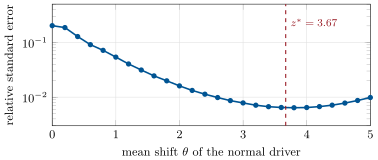
The optimal density needs the answer, but it says where to look: sample in proportion to where the payoff lives. For a digital paying if $S_T > 250$ (probability $1.21 \times 10^{-4}$, the normal driver above $z^* = 3.67$), 100 000 plain draws produce six hits and a relative standard error of 20%. Shifting the driver’s mean to $\theta$ and weighting each draw by $e^{-\theta Z + \theta^2/2}$ brings it to 0.64% at $\theta = 3.8$, a variance factor of about 1 000 (Figure 26.1); shifting too far makes it worse again, as the weights of the few draws that matter explode.

26.3 Low-discrepancy sequences

Definition 26.8 (Low-discrepancy sequence, Sobol sequence, quasi-Monte Carlo)

The star discrepancy $D_n^*$ of points $x_1, \dots, x_n$ in $[0, 1)^d$ is the largest difference, over boxes $[0, a)$, between the fraction of points in the box and its volume. A low-discrepancy sequence has $D_n^* = O((\log n)^d/n)$. The Sobol sequence (Sobol, 1967) is a base-2 low-discrepancy sequence built coordinate by coordinate from primitive polynomials and direction numbers, by exclusive-or of binary digits. Quasi-Monte Carlo replaces the random draws of Monte Carlo by such points.

Proposition 26.9 (Koksma–Hlawka inequality)

For $f$ of bounded variation $V(f)$ in the sense of Hardy and Krause, $\bigl|\frac1n\sum_if(x_i) - \int_{[0,1)^d}f\bigr| \le V(f)\,D_n^*$.

The bound gives quasi-Monte Carlo a rate close to $1/n$ for smooth integrands of moderate effective dimension, but it is a worst-case bound that cannot be estimated from the points. Randomisation restores an error estimate.

Definition 26.10 (Randomised quasi-Monte Carlo, Brownian bridge construction)

Randomised quasi-Monte Carlo randomises a low-discrepancy set so that each point is uniform while the set keeps its structure, and estimates the error from independent replicates. The kit uses Owen’s nested uniform scrambling (1995): each binary digit of each coordinate is flipped by a random bit attached to the node of the binary tree that its leading digits define. The Brownian bridge construction assigns the first coordinate to $W_T$, the next to $W_{T/2}$ given its ends, and so on down the levels, so that the first coordinates, where low-discrepancy points are best, carry most of the variance of the path.

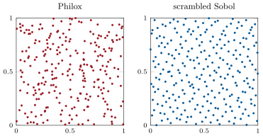
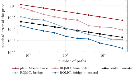
Figure 26.2 shows why: 256 scrambled Sobol points in two dimensions put exactly one point in each of 256 dyadic boxes of every shape, where independent draws leave gaps and clusters. On the average-price call with $2^{14}$ paths and 32 independent scrambles, scrambled Sobol points with the increments in time order reduce the variance by a factor of about 34; with the Brownian bridge construction by about 2 500; with the bridge and the control variate together by about 37 000, a standard error 190 times smaller at the same number of paths. The error also falls faster than $n^{-1/2}$: fitted slopes between $-0.7$ and $-0.8$ from $2^6$ to $2^{15}$ paths (Figure 26.3).

26.4 Discretisation and multilevel methods

Definition 26.11 (Strong and weak orders of convergence, Milstein scheme)

A scheme with step $h$ has strong order of convergence $\gamma$ if $\E|X_T^h - X_T| \le Ch^\gamma$, and weak order of convergence $\beta$ if $|\E g(X_T^h) - \E g(X_T)| \le Ch^\beta$ for smooth $g$. The Milstein scheme for $dX = a(X)\,dt + b(X)\,dW$ adds to the Euler–Maruyama step the term $\frac12b(X)b'(X)((\Delta W)^2 - h)$.

Proposition 26.12 (Orders of Euler and Milstein)

Under Lipschitz and growth conditions (and smoothness of $a$, $b$ for Milstein), the Euler–Maruyama scheme has strong order $\frac12$ and weak order 1, and the Milstein scheme strong order 1 (Kloeden and Platen, 1992).

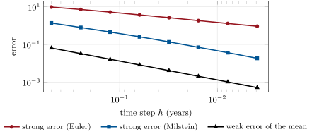
A price needs the weak order; a hedge simulated along the path, or a multilevel estimator, needs the strong one. On a geometric Brownian motion with $\sigma = 50\%$, driven by the same increments as the exact solution, the fitted strong slopes are 0.49 for Euler and 0.89 for Milstein, and the weak error of the mean is exactly $X_0|(1 + \mu h)^n - e^{\mu T}|$, slope 1.00 (Figure 26.4).

Definition 26.13 (Multilevel Monte Carlo)

Multilevel Monte Carlo (Giles, 2008) writes the finest-level expectation as a telescoping sum $\E P_L = \E P_0 + \sum_{l=1}^L\E[P_l - P_{l-1}]$, where $P_l$ is the payoff computed with step $h_l = 2^{-l}T$, and estimates each term independently, with $P_l$ and $P_{l-1}$ in each correction computed from the same Brownian path.

Proposition 26.14 (Complexity of multilevel Monte Carlo)

If the bias of $P_l$ is $O(2^{-\alpha l})$, the variance of the correction $V_l = O(2^{-\beta l})$ and its cost $C_l = O(2^{\gamma l})$, with $\alpha \ge \frac12\min(\beta, \gamma)$, then a mean square error $\epsilon^2$ costs $O(\epsilon^{-2})$ if $\beta > \gamma$, $O(\epsilon^{-2}(\log\epsilon)^2)$ if $\beta = \gamma$ and $O(\epsilon^{-2 - (\gamma - \beta)/\alpha})$ if $\beta < \gamma$; standard Monte Carlo costs $O(\epsilon^{-2 - \gamma/\alpha})$.

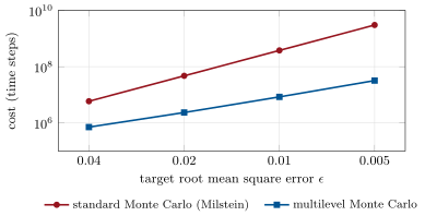
The strong order sets $\beta$: Milstein on a Lipschitz payoff gives $\beta = 2 > \gamma = 1$, and the corrections’ variances in the tutorial fall by a factor of about four per level (0.23, 0.060, 0.016, 0.0045, 0.0012, 0.00030, 0.000079). For a European call ($\alpha = 1$), the driver listed in Section 26.5 reaches a root mean square error of 0.005 with 7 levels at a cost of $3.2 \times 10^7$ time steps, where standard Monte Carlo at the same finest step would need $3.0 \times 10^9$: a factor of 94, which grows as $\epsilon$ falls (8, 20, 45, 94 for $\epsilon$ from 0.04 to 0.005; Figure 26.5).

26.5 Tutorial: sixteen times fewer machines

26.6 Build: the Monte Carlo engine, stage three

26.7 Exercises

Exercise 26.1 ★

A batch has standard error 80 000 dollars with 100 000 paths. How many paths reach 20 000, and what variance-reduction factor does the same at 100 000 paths?

Solution

Solution of Exercise 26.1.

Error scales as $n^{-1/2}$: a factor of four needs $16 \times 100\,000 = 1.6$ million paths, or a variance-reduction factor of 16 at 100 000 paths.

Exercise 26.2 ★

A control variate has correlation 0.9 with the payoff. What is the variance factor? And with 0.99?

Solution

Solution of Exercise 26.2.

$1/(1 - \rho^2)$: 5.3 at $\rho = 0.9$ and 50.3 at $\rho = 0.99$. High correlations are needed for large factors.

Exercise 26.3 ★

Why do antithetic variates help a monotone payoff and not an even function of $Z$ such as $Z^2$?

Solution

Solution of Exercise 26.3.

$\Var(\frac12(f(Z) + f(-Z))) = \frac12\Var f(Z)(1 + \mathrm{Corr}(f(Z), f(-Z)))$ per pair, i.e. per two evaluations; it beats plain sampling when the correlation is negative, which a monotone $f$ guarantees. For an even function $f(Z) = f(-Z)$, the correlation is 1 and the pair is worth one draw at the cost of two.

Exercise 26.4 ★★

Show that proportional stratification never increases the variance: with strata $s$ of probability $p_s$ and conditional variances $\sigma_s^2$, the stratified variance is $\frac1n\sum_sp_s\sigma_s^2 \le \sigma^2/n$.

Solution

Solution of Exercise 26.4.

By the law of total variance, $\sigma^2 = \sum_sp_s\sigma_s^2 + \sum_sp_s(\mu_s - \mu)^2$. The stratified estimator $\sum_sp_s\bar Y_s$ with $n_s = np_s$ has variance $\sum_sp_s^2\sigma_s^2/n_s = \frac1n\sum_sp_s\sigma_s^2$, which drops the nonnegative between-strata term.

Exercise 26.5 ★★

For $P(Z > z^*)$ with $Z$ standard normal, compute the second moment of the importance-sampling estimator with the shift $\theta$, and show that it is minimised near $\theta = z^*$ for large $z^*$.

Solution

Solution of Exercise 26.5.

The estimator is $\mathbf 1\{Z > z^*\}e^{-\theta Z + \theta^2/2}$ with $Z \sim \mathcal N(\theta, 1)$; its second moment is

$$\E_f\bigl[\mathbf 1\{Z > z^*\}e^{-\theta Z + \theta^2/2}\bigr] = e^{\theta^2}\bar\Phi(z^* + \theta).$$

The derivative of its logarithm is $2\theta - \varphi(z^* + \theta)/\bar\Phi(z^* + \theta) \approx 2\theta - (z^* + \theta)$ for large arguments (Mills’s ratio), which vanishes at $\theta \approx z^*$. At $z^* = 3.67$ the exact minimiser is 3.80, where the simulation’s minimum is.

Exercise 26.6 ★★

Derive the Milstein step for geometric Brownian motion and show that it is the second-order expansion of the exact step $X e^{(\mu - \sigma^2/2)h + \sigma\Delta W}$ in $\Delta W$.

Solution

Solution of Exercise 26.6.

With $a(x) = \mu x$ and $b(x) = \sigma x$, $bb' = \sigma^2x$: $X_{k+1} = X_k(1 + \mu h + \sigma\Delta W + \frac12\sigma^2(\Delta W^2 - h))$. Expanding the exact step, $e^{(\mu - \sigma^2/2)h + \sigma\Delta W} = 1 + \sigma\Delta W + (\mu - \frac12\sigma^2)h + \frac12\sigma^2\Delta W^2 + O(h^{3/2})$, the same terms.

Exercise 26.7 ★★★

Coding. Compute the variance factor of the control variate at strikes 80, 100 and 130, and explain the trend.

Solution

Solution of Exercise 26.7.

With $2^{14}$ paths: correlation 0.99953, 0.99941 and 0.99425, variance factors 1 071, 853 and 87 at strikes 80, 100 and 130. Far out of the money the geometric average (always below the arithmetic one) finishes in the money less often than the arithmetic one, and the two payoffs decouple near the strike: the control is worth less where both are rare.

Exercise 26.8 ★★★

Find the flaw. “We moved the batch to Sobol points, 100 000 per trade, and report the standard error $s/\sqrt n$ from the points as before; it fell by a factor of ten.”

Solution

Solution of Exercise 26.8.

Sobol points are not independent, so $s/\sqrt n$ is not the standard error of their average: it measures the spread of the payoffs, not of the estimate, and says nothing about the error, which may be smaller or, with a poor path construction, larger. The error must come from independent scrambles (replicates), and unscrambled points give no error estimate at all.

26.8 Problem: Sixteen Times Fewer Machines

Problem 26.1

Weekend problem — a factor of four in error, without sixteen times the paths

The representative trade is an arithmetic-average call on 64 fixings ($S_0 = K = 100$, $r = 3\%$, $\sigma = 25\%$, one year), valued with $2^{14}$ paths; the batch needs a factor of four in standard error.

Part I — The plain estimator.

1. What are the plain estimate, its standard error and the reference price?
2. What variance factor does the target require?
3. What does the cost-variance product say about comparing estimators?
4. Why does the counter-based generator make the batch reproducible across machines?
5. Why is the inverse transform, rather than Box–Muller, used to feed low-discrepancy points?

Part II — Variance reduction.

6. What factor do antithetic pairs give, and why so little?
7. What is the control variate, its closed-form value, its correlation and its factor?
8. What is the optimal coefficient, and what was estimated?
9. Where does importance sampling help, and by how much on the deep out-of-the-money digital?
10. Why does too large a shift make it worse?

Part III — Points and paths.

11. What factor do scrambled Sobol points give with the increments in time order, and with the bridge?
12. Why does the bridge matter so much?
13. What do the two together give, and what is the error’s slope in the number of paths?
14. How is the error of randomised quasi-Monte Carlo estimated?
15. What do the strong and weak orders measure, and what are their fitted values here?

Part IV — Judgement.

16. What does multilevel Monte Carlo save on the European call at $\epsilon = 0.005$, and why?
17. Would the factor of 37 000 hold across the batch?
18. What must the batch log so that one trade’s paths can be regenerated?
19. State the named result: the variance-reduction factor of the control variate plus randomised quasi-Monte Carlo on the representative trade, against the 16 required.
20. In one sentence: where does the work of a Monte Carlo engine go?

Solution

Solution of Problem 26.1.

1. 6.495 with standard error 0.077 from $2^{14}$ paths; reference 6.4788 (control variate plus scrambled Sobol, 32 replicates of $2^{14}$, standard error 0.00007). 2. 16. 3. At equal accuracy the cost is $c\sigma^2/\epsilon^2$, so estimators are compared by variance times cost per draw; all the factors here are at equal payoff evaluations. 4. Each path’s numbers are a function of (seed, trade, path, block), not of a sequential state, so any split of the paths reproduces them. 5. It maps one uniform coordinate to one normal monotonically, so the structure of the point set survives; Box–Muller mixes two coordinates through a cosine. 6. 1.8: the two payoffs of a pair have correlation $-0.43$; the payoff is monotone in the path but convex, and its positive part discards the down paths. 7. The geometric-average call, 6.1793 in closed form; correlation 0.99941; factor 853. 8. $\beta^* = \Cov(Y, C)/\Var C$; estimated from the same paths as 1.04 (the bias this introduces is of order $1/n$). 9. Where the payoff lives in a small region of the driver’s space: at $\theta = 3.8$ the relative standard error falls from 20% to 0.64%, a factor of about 1 000 in variance. 10. The likelihood ratio $e^{-\theta Z + \theta^2/2}$ becomes very variable: the second moment $e^{\theta^2}\bar\Phi(z^* + \theta)$ grows again beyond the optimum. 11. About 34 with the increments in time order and about 2 500 with the bridge. 12. Low-discrepancy points are most uniform in their first coordinates; the bridge puts $W_T$ and the coarse shape of the path there, the directions that carry most of the payoff’s variance. 13. About 37 000 (standard error 190 times smaller); fitted slopes between $-0.7$ and $-0.8$ against $-0.5$ for Monte Carlo. 14. From the spread of independent scrambles: $R$ replicates give $R$ independent unbiased estimates, whose sample standard deviation divided by $\sqrt R$ is the standard error. 15. Strong: the pathwise error, slopes 0.49 (Euler) and 0.89 (Milstein); weak: the error in law, slope 1.00 for the mean. 16. Cost $3.2 \times 10^7$ time steps against $3.0 \times 10^9$, a factor of 94: most samples are drawn on coarse, cheap levels, and the fine corrections have small variance because Milstein’s strong order 1 makes $V_l$ fall by four per level. 17. No: it relies on a smooth payoff with a closed-form control and a low effective dimension. Barriers, digitals and early exercise break the smoothness, and most trades have no control as good; each trade class must be measured. 18. Seed, trade and path counters, generator and version, scrambling seeds, the path construction, and the point-set size. 19. Named result: sixteen times fewer machines: on the representative trade, the control variate alone reduces the variance by 853 and with scrambled Sobol points and the Brownian bridge by about 37 000, against the 16 required; the target is met at today’s number of paths, with the generation overhead to be measured in the production engine. 20. Into the constant in front of $n^{-1/2}$: what each path is worth, and what it costs.

26.9 Interview questions

Interview question 26.1 ★ researcher, developer

How does the Monte Carlo error scale with the number of paths and with the dimension?

Solution

Solution of Interview question 26.1.

The standard error is $\sigma/\sqrt n$ whatever the dimension: the dimension enters only through $\sigma$ and the cost of a path, which is why Monte Carlo wins in high dimension and loses to grids in one or two.

What the interviewer is looking for: $n^{-1/2}$, dimension-free, the constant.

Interview question 26.2 ★★ researcher

Name three variance-reduction techniques and when each works.

Solution

Solution of Interview question 26.2.

Antithetic variates (monotone payoffs, cheap, small gains); control variates (a correlated quantity with known mean: the geometric Asian, the underlying, a Black–Scholes price); importance sampling (rare events: shift the drift towards the region that matters); stratification or quasi-Monte Carlo (smooth payoffs in a few important directions).

What the interviewer is looking for: When each works, not just names.

Interview question 26.3 ★★ developer

How do you make a distributed Monte Carlo batch reproducible regardless of the number of machines?

Solution

Solution of Interview question 26.3.

Use a counter-based generator (Philox, Threefry) keyed by the seed, with the counter built from trade, path and block indices, so that numbers are a function of their coordinates, not of the order of generation; reduce partial sums in a fixed order.

What the interviewer is looking for: Counters over sequential streams, and a fixed reduction order.

Interview question 26.4 ★★ researcher

Why might quasi-Monte Carlo do badly on a 250-step path, and what fixes it?

Solution

Solution of Interview question 26.4.

Its uniformity is good only in the first coordinates, and in time order the path’s variance is spread evenly over 250 of them. Fix it with a Brownian bridge or principal-component construction that puts the important directions first, and scramble to get error estimates.

What the interviewer is looking for: Effective dimension and path construction.

Interview question 26.5 ★★ researcher, risk

How would you estimate the probability of a loss beyond a very high threshold by simulation?

Solution

Solution of Interview question 26.5.

Importance sampling: tilt the distribution (shift the mean of the drivers, or exponentially tilt the loss) so that the loss beyond the threshold is common, and weight by the likelihood ratio; choose the tilt near the most likely point of the rare region; check the weights’ spread. Splitting or conditional Monte Carlo are alternatives.

What the interviewer is looking for: A change of measure with the likelihood ratio, and a sensible choice of tilt.

Interview question 26.6 ★★★ researcher

Explain multilevel Monte Carlo and why the strong order of the scheme matters for it.

Solution

Solution of Interview question 26.6.

Write the finest-level expectation as a telescoping sum of corrections between successive step sizes, simulate the fine and coarse paths of each correction from the same Brownian path, and allocate samples in proportion to $\sqrt{V_l/C_l}$. The correction’s variance $V_l$ is governed by the strong error, so a higher strong order makes the fine levels need very few samples; with $V_l$ falling faster than the cost rises, the total cost is $O(\epsilon^{-2})$, as for an unbiased estimator.

What the interviewer is looking for: Telescoping sum, coupling, and the variance of corrections from the strong order.