3Itô Calculus

A junior researcher backtests a trend-following rule on ten years of daily closes: hold a position proportional to the distance of the close above its 20-day moving average. The Sharpe ratio is 5.4. The rule reads the closing price and the backtest credits it with the return into that same close; shifted by one day, so that a position decided at a close earns the next day’s return, the Sharpe ratio is $-0.04$. The “prices” were a pure random walk, with nothing to find. The first backtest was not an Itô integral: its integrand looked at the increment it was multiplied by, and collected the covariation of the position with the price, a quantity that exists on every random path. This chapter builds the Itô integral, whose integrand is fixed before the increment arrives, proves Itô’s formula, the chain rule with a second-order term that the rest of the series uses on every page, and ends with the two structural theorems (Lévy’s characterisation and martingale representation) that underlie the pricing of One Quant Book 5.

3.1 The Itô integral

A trading strategy holds $H_t$ units of an asset whose price follows a Brownian motion; its gains over $[0, T]$ should be $\int_0^T H_t\,dW_t$. The paths of $W$ have infinite total variation (Theorem 2.12), so the integral cannot be defined path by path as a Stieltjes integral, and the choice of evaluation point in each interval matters in the limit. The Itô integral evaluates $H$ at the left point, which is the only choice a trader can make.

Definition 3.1 (Simple process, Itô integral)

A simple process is $H_t = \sum_{k=0}^{n-1}h_k\mathbf 1_{(t_k, t_{k+1}]}(t)$ with $0 = t_0 < \dots < t_n = T$ and each $h_k$ bounded and $\mathcal F_{t_k}$-measurable. Its Itô integral is $\int_0^t H_s\,dW_s = \sum_k h_k(W_{t_{k+1}\wedge t} - W_{t_k\wedge t})$. For an adapted $H$ with $\E\int_0^T H_s^2\,ds < \infty$, the Itô integral is the $L^2$ limit of the integrals of simple processes $H^{(n)}$ with $\E\int_0^T(H^{(n)}_s - H_s)^2\,ds \to 0$.

Theorem 3.2 (Itô isometry)

For adapted $H$ with $\E\int_0^T H_s^2\,ds < \infty$, $I_t = \int_0^t H_s\,dW_s$ is a continuous square-integrable martingale with $I_0 = 0$ and

$$\E\Bigl[\Bigl(\int_0^T H_s\,dW_s\Bigr)^2\Bigr] = \E\int_0^T H_s^2\,ds, \qquad [I]_t = \int_0^t H_s^2\,ds.$$

Example 3.3 (The integral of $W$ against itself)

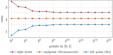
On a partition of $[0, T]$, $\sum_k W_{t_k}\Delta_k = \tfrac12\sum_k(W_{t_{k+1}}^2 - W_{t_k}^2) - \tfrac12\sum_k\Delta_k^2$. The first sum telescopes to $\tfrac12 W_T^2$ and the second tends to $\tfrac12 T$ by Theorem 2.12:

$$\int_0^T W_t\,dW_t = \tfrac12\bigl(W_T^2 - T\bigr).$$

The right-point sums tend to $\tfrac12(W_T^2 + T)$, and the midpoint sums to $\tfrac12W_T^2$, the ordinary calculus answer (Figure 3.1).

Definition 3.4 (Stratonovich integral)

The Stratonovich integral $\int_0^T X_t\circ dW_t$ is the limit of the sums $\sum_k\tfrac12(X_{t_k} + X_{t_{k+1}})\Delta_k$. For a continuous semimartingale $X$ it equals $\int_0^T X_t\,dW_t + \tfrac12[X, W]_T$.

The Stratonovich integral obeys the ordinary chain rule, which is why physicists modelling a smooth noise by a white one use it. It averages the integrand over the interval, which a trade cannot do: the position is set before the price move. Finance uses Itô.

3.2 The integral in a backtest

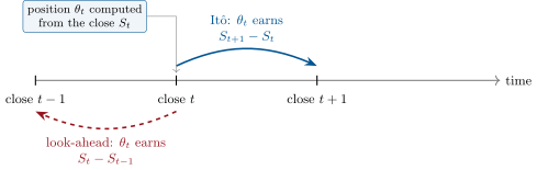
A backtest on a grid $t_0 < t_1 < \dots$ with positions $\theta_{t_i}$ and prices $S_{t_i}$ computes gains $\sum_i\theta_{t_i}(S_{t_{i+1}} - S_{t_i})$: the left-point sum, an Itô integral, when $\theta_{t_i}$ uses only information available at $t_i$. A backtest that credits the position computed at $t_{i+1}$ with the move into $t_{i+1}$ computes the right-point sum instead, and

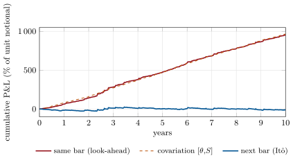
the look-ahead profit is the covariation of the position with the price, which is not zero on a random walk whenever the position responds to the latest price. The rule of the hook, $\theta_t = (S_t - \bar S^{(20)}_t)/c$ with $\bar S^{(20)}$ the 20-day moving average and $c$ chosen so that $\theta$ has unit variance, puts weight $(L - 1)/L = 0.95$ on the last increment: Figure 3.2 shows the timing and Figure 3.3 the result.

Proposition 3.5 (The look-ahead Sharpe ratio on a random walk)

Let $S$ be a random walk with daily increments $\sigma Z_t$, $Z_t$ independent standard normal, and $\theta_t$ a unit-variance linear function of past increments with correlation $a$ with the latest one. Then the same-bar gains $\theta_t\,\Delta S_t$ have mean $a\sigma$ and standard deviation $\sigma\sqrt{1 + a^2}$, a daily Sharpe ratio of $a/\sqrt{1 + a^2}$, while the next-bar gains have mean zero. For the moving-average rule, $a = \frac{(L-1)/L}{(\sum_{m=1}^{L-1}(m/L)^2)^{1/2}}$.

For $L = 20$, $a = 0.382$ and the annualised same-bar Sharpe ratio is $\sqrt{252}\times 0.382/ \sqrt{1.146} = 5.67$; over 400 simulated ten-year random walks it averages 5.69, and the honest backtest 0.00 with a standard deviation of 0.32, the noise one expects from ten years of a strategy with no edge.

3.3 Itô’s formula in one and several dimensions

Definition 3.6 (Itô process, quadratic covariation)

An Itô process is $X_t = X_0 + \int_0^t\mu_s\,ds + \int_0^t\sigma_s\,dW_s$, written $dX_t = \mu_t\,dt + \sigma_t\,dW_t$, with adapted $\mu$, $\sigma$ such that $\int_0^T|\mu_s|\,ds$ and $\int_0^T\sigma_s^2\,ds$ are finite almost surely. The quadratic covariation of two continuous processes is the limit in probability $[X, Y]_t = \lim\sum_k(X_{t_{k+1}} - X_{t_k})(Y_{t_{k+1}} - Y_{t_k})$; for Itô processes driven by $W^1, W^2$ with $d\langle W^1, W^2\rangle_t = \rho\,dt$, $d[X, Y]_t = \sigma^X_t\sigma^Y_t\rho\,dt$.

The bookkeeping rules are $dt\,dt = 0$, $dt\,dW = 0$, $dW^i\,dW^j = \rho_{ij}\,dt$: only products of two Brownian increments survive at first order in $dt$.

Theorem 3.7 (Itô’s formula)

If $X$ is an Itô process and $f \in C^{1,2}([0,T]\times\R)$, then

$$df(t, X_t) = \partial_tf\,dt + \partial_xf\,dX_t + \tfrac12\partial_{xx}f\,d[X]_t = \bigl(\partial_tf + \mu_t\partial_xf + \tfrac12\sigma_t^2\partial_{xx}f\bigr)dt + \sigma_t\partial_xf\,dW_t.$$

For $X = (X^1, \dots, X^d)$ and $f \in C^{1,2}$, $df = \partial_tf\,dt + \sum_i\partial_if\,dX^i + \tfrac12\sum_{i,j}\partial_{ij}f\,d[X^i, X^j]$; in particular $d(XY) = X\,dY + Y\,dX + d[X, Y]$.

Example 3.8 (The logarithm of a geometric Brownian motion)

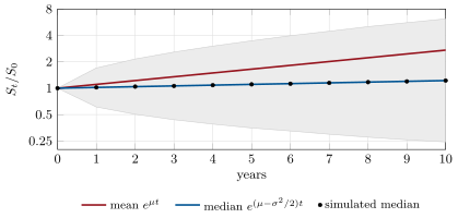
For $dS = \mu S\,dt + \sigma S\,dW$, with $f = \ln$: $d\ln S = dS/S - \tfrac12 d[S]/S^2 = (\mu - \tfrac12\sigma^2)dt + \sigma\,dW$. The expected return is $\mu$ but the expected log return, the rate at which the median grows, is $\mu - \tfrac12\sigma^2$. With $\mu = 10\%$ and $\sigma = 40\%$, the mean of $S_{10}/S_0$ is $e^{1} = 2.72$ and its median $e^{0.2} = 1.22$ (Figure 3.4); the volatility decay of leveraged funds (One Quant Book 1, chapter 14) is the same correction applied twice.

3.4 Local martingales and the stochastic exponential

An Itô integral $\int H\,dW$ with only $\int_0^TH_s^2\,ds < \infty$ almost surely need not be integrable, let alone a martingale; it is one up to a sequence of stopping times.

Definition 3.9 (Local martingale)

An adapted process $M$ is a local martingale if there are stopping times $\tau_n \uparrow \infty$ such that each stopped process $M_{t\wedge\tau_n}$ is a martingale.

Proposition 3.10 (Positive local martingales are supermartingales)

A local martingale bounded below, in particular a positive one, is a supermartingale. A local martingale $M$ with $\E[\sup_{s\le t}|M_s|] < \infty$ for every $t$ is a martingale.

The inequality can be strict: $1/|B_t|$ for a three-dimensional Brownian motion started away from the origin is a positive local martingale whose expectation decreases, a strict local martingale. Such processes model price bubbles and are why chapter 5 checks that a candidate density process is a true martingale before using it to change the measure.

Definition 3.11 (Stochastic exponential)

The stochastic exponential of a continuous semimartingale $X$ with $X_0 = 0$ is $\mathcal E(X)_t = \exp(X_t - \tfrac12[X]_t)$, the unique solution of $dZ = Z\,dX$, $Z_0 = 1$.

By Itô’s formula, $d\exp(X - \tfrac12[X]) = \exp(\cdot)(dX - \tfrac12 d[X] + \tfrac12 d[X]) = Z\,dX$. With $X = \int\gamma\,dW$ it is the positive local martingale $\exp(\int\gamma\,dW - \tfrac12\int\gamma^2dt)$, the density process of every change of measure in chapter 5.

3.5 The representation theorem

Theorem 3.12 (Lévy’s characterisation)

A continuous local martingale $M$ with $M_0 = 0$ and $[M]_t = t$ is a Brownian motion.

Theorem 3.13 (Martingale representation)

Let $\mathbb F$ be the filtration generated by a Brownian motion $W$. Every square-integrable $\mathbb F$-martingale $M$ has the form $M_t = M_0 + \int_0^tH_s\,dW_s$ for a unique adapted $H$ with $\E\int_0^TH_s^2\,ds < \infty$.

Both are proved in Karatzas and Shreve (1991, §3.3 and §3.4). The representation theorem is the mathematics of replication: if the only randomness is $W$, every payoff’s conditional expectation is a stochastic integral against $W$, and $H$ is the position that reproduces it. One Quant Book 5, chapter 1, builds on it the notions of a replicating portfolio and a complete market; it fails as soon as there are jumps (chapter 6) or more sources of risk than traded assets.

3.6 Tutorial: Itô sums and an honest backtest

3.7 Build: discrete stochastic integrals

3.8 Exercises

Exercise 3.1 ★

Compute $\E[(\int_0^1W_t\,dW_t)^2]$ with the isometry and check it with Example 3.3.

Solution

Solution of Exercise 3.1.

$\E\int_0^1W_t^2\,dt = \int_0^1t\,dt = \tfrac12$. With Example 3.3, $\Var(\tfrac12(W_1^2 - 1)) = \tfrac14\Var(W_1^2) = \tfrac14 \times 2 = \tfrac12$, and the mean is zero.

Exercise 3.2 ★

Write $d(W_t^3)$ with Itô’s formula, and deduce $\E[W_t^3]$ and a martingale built from $W^3$.

Solution

Solution of Exercise 3.2.

$d(W^3) = 3W^2\,dW + 3W\,dt$. Taking expectations, $\E[W_t^3] = 3\int_0^t\E[W_s]\,ds = 0$, and $W_t^3 - 3\int_0^tW_s\,ds$ is a martingale.

Exercise 3.3 ★

A stock follows a geometric Brownian motion with $\mu = 10\%$ and $\sigma = 40\%$. What are the mean and the median of $S_{10}/S_0$, and at what volatility would the median not grow at all?

Solution

Solution of Exercise 3.3.

Mean $e^{1} = 2.72$, median $e^{(0.10 - 0.08) \times 10} = 1.22$. The median is flat when $\sigma^2 = 2\mu$, $\sigma = \sqrt{0.2} = 44.7\%$.

Exercise 3.4 ★★

Show that $e^{W_t - t/2}$ is a martingale and compute $\E[e^{2W_1}]$.

Solution

Solution of Exercise 3.4.

It is $\mathcal E(W)_t$: $dZ = Z\,dW$, and $\E\int_0^tZ_s^2\,ds = \int_0^te^s\,ds < \infty$, so the Itô integral is a true martingale. $\E[e^{2W_1}] = e^{2}= 7.39$ (the moment generating function of $\mathcal N(0,1)$ at 2).

Exercise 3.5 ★★

Use the product rule on $tW_t$ to write $\int_0^1 W_t\,dt$ as a stochastic integral, and compute its variance.

Solution

Solution of Exercise 3.5.

$d(tW_t) = W_t\,dt + t\,dW_t$, so $\int_0^1W_t\,dt = W_1 - \int_0^1t\,dW_t = \int_0^1(1 - t)\,dW_t$, with variance $\int_0^1(1 - t)^2dt = \tfrac13$ by the isometry.

Exercise 3.6 ★★

$X = W^1$ and $Y = 2W^1 + W^2$ with $W^1, W^2$ independent. Compute $[X, Y]_t$, $[Y]_t$ and the instantaneous correlation of $X$ and $Y$.

Solution

Solution of Exercise 3.6.

$[X, Y]_t = 2t$, $[Y]_t = 5t$, correlation $2/\sqrt5 = 0.894$.

Exercise 3.7 ★★★

Coding. Repeat the backtest with a 60-day moving average: compute the look-ahead Sharpe ratio from Proposition 3.5 and its average over 100 simulated ten-year walks.

Solution

Solution of Exercise 3.7.

$L = 60$ gives $a = 0.223$ and a look-ahead Sharpe ratio of 3.45; the average over 100 seeded walks is 3.47. A slower average puts less weight on the last increment, so the bias is smaller, but it is still enormous.

Exercise 3.8 ★★★

Find the flaw. “Our rule decides from the closing price and trades in the closing auction; the backtest credits it with the next day’s return, so there is no look-ahead.”

Solution

Solution of Exercise 3.8.

The signal uses the closing price, which is not known until the closing auction in which the rule claims to trade has printed: the decision is not adapted to the information available when the order must be sent. Compute the signal from the auction’s indicative price published before the order deadline (chapter 1), or trade at the next open.

3.9 Problem: The Look-Ahead in the Backtest

Problem 3.1

Weekend problem — a Sharpe ratio of 5.4 on a random walk

The log price is a random walk with 1% daily volatility. The rule holds $\theta_t = (S_t - \bar S^{(20)}_t)/c$, with $c$ making $\theta$ of unit variance; the flawed backtest credits $\theta_t$ with $S_t - S_{t-1}$, the honest one with $S_{t+1} - S_t$.

Part I — The rule.

1. What is $c$?
2. What is the correlation $a$ of $\theta_t$ with the day’s increment?
3. What are the mean and standard deviation of the same-bar gain per day?
4. What is the annualised same-bar Sharpe ratio?
5. What does the honest backtest earn on average, and why?

Part II — The simulation.

6. What Sharpe ratios does the seeded ten-year history give for the two backtests?
7. Over 400 histories, what are the mean and standard deviation of each?
8. Check the identity same-bar $-$ honest $=$ covariation on the seeded history.
9. What $t$-statistic does lookahead_test report for the seeded history?
10. Why is the honest Sharpe ratio’s standard deviation about $1/\sqrt{10}$?

Part III — The Itô view.

11. Write the same-bar P&L as an Itô integral plus a covariation.
12. Why is the expectation of the Itô part zero?
13. What are the look-ahead Sharpe ratios for windows of 5, 10 and 60 days?
14. If the flawed backtest ran on five-minute bars, 78 a day, with the same rule in bars, what would its annualised Sharpe ratio be?
15. Would trading at the next day’s open instead of the close remove the bias?

Part IV — Judgement.

16. How would you detect this error in someone else’s backtest?
17. Is look-ahead bias always positive?
18. On real prices with a bid–ask bounce, what else can produce a covariation between position and price?
19. State the named result: the look-ahead Sharpe ratio of the same-bar trend rule on a random walk.
20. In one sentence: what makes a backtest an Itô integral?

Solution

Solution of Problem 3.1.

1. $c = 0.01\,(\sum_{m=1}^{19}(m/20)^2)^{1/2} = 0.01 \times 2.485 = 0.0248$. 2. $a = 0.95/2.485 = 0.382$. 3. Mean $a\sigma = 0.0038$ and standard deviation $\sigma\sqrt{1 + a^2} = 0.0107$ per day, per unit of position. 4. $\sqrt{252} \times 0.382/1.070 = 5.67$. 5. Zero: $\theta_{t}$ is independent of $S_{t+1} - S_t$. 6. 5.43 same-bar, $-0.04$ next-bar. 7. Same-bar $5.69 \pm 0.13$; next-bar $0.00 \pm 0.32$. 8. Both equal 9.653 (965% of notional); the difference is $2 \times 10^{-14}$. 9. 34.9. 10. With no edge the annualised Sharpe ratio estimated over $T$ years has a standard error of about $1/\sqrt T$ (chapter 11): $0.32$ for ten years. 11. $\sum\theta_t\Delta S_t = \sum\theta_{t-1}\Delta S_t + \sum\Delta\theta_t\Delta S_t$: an Itô sum plus the covariation $[\theta, S]$. 12. Its integrand is adapted, so it is a martingale started at zero. 13. 9.36, 7.47 and 3.45. 14. The daily Sharpe ratio per bar is unchanged, and annualising over $252 \times 78$ bars multiplies it by $\sqrt{78}$: 50. 15. Yes, if the signal uses only the close and the gains start at the next open; the position then misses the overnight move, which the honest backtest must also leave out. 16. Shift the positions by one bar and see whether the performance collapses; run lookahead_test, or regress the daily P&L on $\Delta\theta_t\Delta S_t$; and read the timestamps of the signal’s inputs. 17. No: its sign is the sign of $[\theta, S]$; a mean-reversion rule, which sells as the price rises, has a negative look-ahead bias. 18. The bounce between bid and ask makes last-trade prices mean-revert; an honest mean-reversion rule on those prices “earns” the bounce, which costs the spread to capture (One Quant Book 10). 19. Named result: the look-ahead in the backtest: on a random walk the same-bar backtest of a unit-variance rule with correlation $a$ to the latest increment has a daily Sharpe ratio $a/\sqrt{1 + a^2}$; for the 20-day trend rule, $a = 0.382$ and the annualised Sharpe ratio is 5.67 (5.69 in simulation), against zero for the Itô sum. 20. Each position is fixed from information available before the price move it is multiplied by.

3.10 Interview questions

Interview question 3.1 ★ researcher

Compute $\int_0^TW_t\,dW_t$. Why is it not $\tfrac12W_T^2$?

Solution

Solution of Interview question 3.1.

$\tfrac12(W_T^2 - T)$. The left-point sums differ from $\tfrac12\sum\Delta(W^2)$ by $\tfrac12\sum(\Delta W)^2$, which tends to $T$: the quadratic variation does not vanish.

What the interviewer is looking for: the telescoping identity and the quadratic variation.

Interview question 3.2 ★ trader, researcher

A stock has an expected return of 10% and a volatility of 40%. What is its expected log return, and what does a typical holder earn over ten years?

Solution

Solution of Interview question 3.2.

$\mu - \sigma^2/2 = 2\%$ a year. The mean of $S_{10}/S_0$ is $e^{1} = 2.72$ but the median is $1.22$, and a tenth of holders end below 0.24: the mean is carried by a few large outcomes.

What the interviewer is looking for: Itô’s correction and mean versus median.

Interview question 3.3 ★★ researcher

Is $W_t^2$ a martingale? Find the process you must subtract, and the variance of $\int_0^TW\,dW$.

Solution

Solution of Interview question 3.3.

No: $d(W^2) = 2W\,dW + dt$, so $W_t^2 - t$ is the martingale. $\Var(\int_0^TW\,dW) = \int_0^Tt\,dt = T^2/2$.

What the interviewer is looking for: Itô’s formula and the isometry.

Interview question 3.4 ★★ developer, researcher

How would you design a backtesting engine that cannot commit look-ahead by construction?

Solution

Solution of Interview question 3.4.

Drive it by events in time order: every datum carries the time it became available, the strategy sees an as-of view, and an order it emits at $t$ can fill only against prices after $t$ plus a latency. The engine, not the strategy, applies positions to the next interval, and a test compares every run with a shifted run and flags covariation between positions and concurrent returns.

What the interviewer is looking for: availability timestamps, as-of joins, and a structural shift.

Interview question 3.5 ★★ researcher, bank

What is a local martingale that is not a martingale, and why should a pricing quant care?

Solution

Solution of Interview question 3.5.

A process that is a martingale only up to a sequence of stopping times; a positive one is a supermartingale and may lose expectation, like $1/|B_t|$ for a three-dimensional Brownian motion. A candidate density for a change of measure, or a deflated price, that is a strict local martingale gives prices that violate put–call parity or a measure that is not a probability.

What the interviewer is looking for: localisation, Fatou, and the pricing consequence.

Interview question 3.6 ★★★ researcher, mle

Itô or Stratonovich: which does finance use, which does physics use, and why?

Solution

Solution of Interview question 3.6.

Finance uses Itô: a position must be set before the price move, which is the left point, and the resulting gains are martingales under the right measure. Physics often uses Stratonovich, the limit of smooth noise, because it keeps the ordinary chain rule. They differ by $\tfrac12[X,W]$.

What the interviewer is looking for: non-anticipation versus smooth-noise limits.