15Robust Statistics and Heavy Tails

One bad print in the feed, the euro’s reference rate recorded as 1.5172 dollars instead of 1.1572 on one day in March 2026, multiplies the standard deviation of the last 250 daily EUR/USD returns by seven, from 0.34% to 2.43%, and moves their median absolute deviation by 1%. A risk system that estimates volatility with the standard deviation now reports a currency as volatile as a small biotechnology stock; one that uses the median absolute deviation has not noticed. The same data hold a second lesson: over 27 years EUR/USD moved more than four standard deviations in a day seventeen times, where a normal law expects fewer than one. This chapter is about estimators that bad data cannot capture and about the tails that good data do contain: the influence function and the breakdown point, winsorising and ranks, copulas and tail dependence, heavy tails and the extreme-value theory that extrapolates them, and the estimation of the tail index on real exchange rates.

15.1 Robust losses and the influence function

Definition 15.1 (Influence function, breakdown point)

For an estimator written as a functional $T(F)$ of the data’s law, the influence function at $x$ is $\mathrm{IF}(x) = \lim_{\varepsilon \to 0}\bigl(T((1 - \varepsilon)F + \varepsilon\delta_x) - T(F)\bigr)/\varepsilon$: the effect on the estimate of an infinitesimal contamination at the point $x$ (Hampel, 1974). The breakdown point is the smallest fraction of the sample that, replaced by arbitrary values, can carry the estimate arbitrarily far.

The mean has $\mathrm{IF}(x) = x - \mu$, unbounded; the variance has $(x - \mu)^2 - \sigma^2$, worse. One observation placed far enough moves either wherever it likes.

Proposition 15.2 (Breakdown points of the mean and the median)

The sample mean has breakdown point $1/n$, which tends to 0; the sample median has breakdown point $\lfloor(n + 1)/2\rfloor/n$, which tends to $1/2$, the largest possible for an equivariant location estimator.

Definition 15.3 (Huber loss, median absolute deviation)

The Huber loss with threshold $c$ is $\rho_c(r) = r^2/2$ for $|r| \le c$ and $c|r| - c^2/2$ otherwise; the Huber M-estimator of location minimises $\sum_i\rho_c((x_i - \mu)/s)$ for a robust scale $s$, so its estimating function $\psi_c(r) = \max(-c, \min(c, r))$ is bounded (Huber, 1964). The median absolute deviation is $\mathrm{MAD} = 1.4826\,\mathrm{med}_i|x_i - \mathrm{med}_jx_j|$, the constant making it consistent for the standard deviation of a normal law.

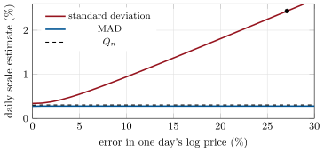
The Huber estimator is the mean near the centre and the median in the tails. With $c = 1.345$ it keeps 95% of the mean’s efficiency when the data are normal ($(2\Phi(c) - 1)^2/\E[\psi_c(Z)^2]$), and its influence function is $\psi_c$, bounded by $c$ standard units. The MAD has breakdown point one half but is inefficient and assumes symmetry; the $Q_n$ estimator of Rousseeuw and Croux (1993), a scaled lower quartile of all pairwise distances $|x_i - x_j|$, keeps the breakdown point without the symmetry. Figure 15.1 shows what the influence functions mean for one bad print: as the error on one day’s log price grows from 0 to 27%, the 250-day standard deviation grows without limit, while the MAD and $Q_n$ move once, by 1.3% and 1.5%, and then not at all.

15.2 Winsorising, trimming and rank methods

Definition 15.4 (Winsorisation, trimmed mean)

Winsorisation at level $p$ replaces the observations below the $p$-quantile by that quantile and those above the $(1 - p)$-quantile by that one. The $p$-trimmed mean discards the $\lfloor pn\rfloor$ smallest and largest observations and averages the rest.

Both have breakdown point $p$. Winsorising is the common repair for a cross-section of signals or returns before a regression (chapter 16): it keeps every observation’s sign and rank and caps its leverage. It is also a decision about the data that the report must state, because a winsorised Sharpe ratio is not the strategy’s Sharpe ratio. For a bad print, the better repair is upstream: filtering clearly erroneous trades against a robust band around a robust centre before any statistic is computed.

Definition 15.5 (Rank correlation, Spearman’s rho, Kendall’s tau)

A rank correlation measures dependence through the ranks of the observations only, so that it is unchanged by increasing transformations of either variable. Spearman’s rank correlation is the correlation of the ranks. Kendall’s tau is the probability that two independent pairs are concordant minus the probability that they are discordant, $\tau = \E[\operatorname{sign}((X - X')(Y - Y'))]$.

Definition 15.6 (Copula, tail dependence coefficient)

A copula is a joint distribution function on $[0, 1]^d$ with uniform margins. The lower tail dependence coefficient of $(X, Y)$ with continuous margins $F_X, F_Y$ is $\lambda_L = \lim_{q \downarrow 0}\P(F_Y(Y) \le q \mid F_X(X) \le q)$, and the upper one is defined symmetrically.

Theorem 15.7 (Sklar)

Every joint distribution function $H$ with margins $F_1, \dots, F_d$ can be written $H(x_1, \dots, x_d) = C(F_1(x_1), \dots, F_d(x_d))$ for a copula $C$, unique when the margins are continuous; conversely, any copula and any margins define a joint law this way.

For continuous margins the proof is one line: $C$ is the law of $(F_1(X_1), \dots, F_d(X_d))$, whose margins are uniform. The theorem separates what a joint law says about each variable from what it says about their dependence, and rank correlations and tail dependence are properties of the copula alone. For the Gaussian copula with correlation $\rho$, Spearman’s rho is $\frac6\pi\arcsin\frac\rho2$, Kendall’s tau $\frac2\pi\arcsin\rho$, and both tail dependence coefficients are zero: joint crashes become asymptotically independent, however high $\rho$ is. Credit portfolio models inherit that property from the Gaussian copula, a point One Quant Book 6 takes up with the Student-$t$ copula, whose tail dependence is positive.

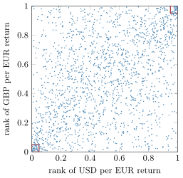
The dollar and the pound, both priced in euros, have a daily Pearson correlation of 0.42 over 1999–2026. Spearman’s rho is 0.406, exactly what a Gaussian copula with that correlation implies (0.406), and Kendall’s tau 0.286 against an implied 0.277. The tails disagree: on the 5% of days when the dollar fell most against the euro, the pound was in its own worst 5% on 32% of them, against 20% for the Gaussian copula; at 1%, 21% against 10% (Figure 15.2). The average dependence is Gaussian; the joint extremes are not.

15.3 Heavy tails

Definition 15.8 (Heavy-tailed distribution, tail index)

A distribution is heavy-tailed (in the Pareto sense) if $\P(X > x) = x^{-\alpha}L(x)$ for a slowly varying $L$ ($L(tx)/L(x) \to 1$ as $x \to \infty$ for every $t > 0$). The exponent $\alpha > 0$ is its tail index.

Proposition 15.9 (Moments beyond the tail index)

If $X \ge 0$ has tail index $\alpha$, then $\E[X^\beta] < \infty$ for $\beta < \alpha$ and $\E[X^\beta] = \infty$ for $\beta > \alpha$.

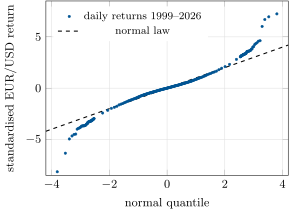
A Student $t$ with $\nu$ degrees of freedom has tail index $\nu$. Mandelbrot’s 1963 study of cotton prices proposed stable laws, whose variance is infinite; the Hill plot below gives EUR/USD’s daily losses a tail index near four, so a finite variance and an unreliable fourth moment, in line with Cont’s survey of stylised facts, which finds tail indices above two and below five for most return series studied. The practical consequence is that the kurtosis, a fourth moment, is estimated badly or not at all: EUR/USD’s sample kurtosis over 27 years is 6.3, and a few days decide it. A quantile-quantile plot shows the tails directly (Figure 15.3).

15.4 Extreme-value theory

Definition 15.10 (Extreme-value theory, GEV distribution)

Extreme-value theory studies the laws of maxima and of exceedances of high thresholds. The generalised extreme value distribution with shape $\xi$ has distribution function $G_\xi(x) = \exp\bigl(-(1 + \xi x)^{-1/\xi}\bigr)$ for $1 + \xi x > 0$ (and $\exp(-e^{-x})$ for $\xi = 0$), up to location and scale.

Theorem 15.11 (Fisher–Tippett–Gnedenko)

If, for iid $X_i$ and constants $a_n > 0$, $b_n$, the law of $(\max_{i \le n}X_i - b_n)/a_n$ converges to a non-degenerate limit, that limit is a generalised extreme value distribution. Heavy tails with index $\alpha$ give $\xi = 1/\alpha > 0$; normal, exponential and similar tails give $\xi = 0$; bounded tails give $\xi < 0$.

Definition 15.12 (Generalised Pareto distribution, peaks over threshold)

The generalised Pareto distribution with shape $\xi$ and scale $\beta$ has $\P(Y > y) = (1 + \xi y/\beta)^{-1/\xi}$ for $y \ge 0$ (and $e^{-y/\beta}$ for $\xi = 0$). The peaks-over-threshold method fits it by maximum likelihood to the excesses $X - u$ of the observations above a high threshold $u$.

Theorem 15.13 (Pickands–Balkema–de Haan)

For a distribution in the domain of attraction of $G_\xi$, the law of the excess $X - u$ given $X > u$ is approximated, uniformly in the excess, by a generalised Pareto law with shape $\xi$ and some scale $\beta(u)$, the error vanishing as $u$ tends to the upper end of the support.

The theorem licenses an extrapolation: with $N_u$ of $n$ observations above $u$, the loss exceeded with probability $1 - p$ is

For EUR/USD daily losses above their 95% quantile ($u = 0.93\%$, 355 excesses), maximum likelihood gives $\xi = 0.069$ and $\beta = 0.34\%$, and the one-in-a-thousand-days loss is 2.47%. The fitted $\xi$ depends on the threshold (0.03 above the 90% quantile, 0.21 above the 99%), the quantile much less (2.43% to 2.49% over the same thresholds): the extrapolation is steadier than the parameter.

15.5 Estimating the tail index

Definition 15.14 (Hill estimator)

With the order statistics $X_{(1)} \ge X_{(2)} \ge \dots$ of a positive sample, the Hill estimator of the tail index from the $k$ largest is $\hat\alpha_k = \bigl(\frac1k\sum_{i=1}^k\ln X_{(i)} - \ln X_{(k+1)}\bigr)^{-1}$ (Hill, 1975).

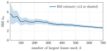
It is the maximum likelihood estimator of $\alpha$ for an exact Pareto tail above $X_{(k+1)}$, and when $k \to \infty$ with $k/n \to 0$ at a suitable rate, $\sqrt k(\hat\alpha_k - \alpha) \to \mathcal N(0, \alpha^2)$. The choice of $k$ is a bias-variance trade: small $k$ is noisy, large $k$ reaches into the body of the law, where the Pareto form fails. The Hill plot shows the trade (Figure 15.4): for EUR/USD losses, $\hat\alpha$ is 4.9 at $k = 50$ ($\pm 0.7$), near 3.9 from $k = 100$ to 200, and drifts down to 2.6 at $k = 700$, where the body is being fitted.

Three models then answer the risk manager’s question, the one-in-a-thousand-days loss (Figure 15.5). The normal law with the sample volatility of 0.58% puts it at 1.80%, and 35 days of the 7 098 lost more, against 7 expected. A Student $t$ fitted by maximum likelihood ($\nu = 4.7$, scale 0.44%) puts it at 2.74%. The generalised Pareto fit puts it at 2.47%, exceeded on 6 days; the empirical quantile is 2.27%.

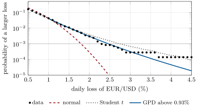
Now put the bad print of the hook into the full history. The normal quantile rises to 2.27% (+26%), because one pair of $\pm 27\%$ returns inflates the standard deviation by a quarter. The generalised Pareto quantile rises to 2.85% (+15%): the bad loss is the largest excess by far and lifts the fitted shape from 0.07 to 0.22. The Student $t$ moves least, to 2.91% (+6%), its likelihood bounding the influence of any single point. No tail estimate is robust in the sense of the first section; the tail is where the information is scarce, and one observation is a large share of it. The defence is upstream, in the filter.

15.6 Tutorial: the bad tick

15.7 Build: the robust statistics module

15.8 Exercises

Exercise 15.1 ★

What are the breakdown points of the 10%-trimmed mean and of the interquartile range?

Solution

Solution of Exercise 15.1.

10% for the trimmed mean (more than the trimmed share on one side carries it away); 25% for the interquartile range, which depends only on the quartiles.

Exercise 15.2 ★

A Pareto tail has index 3. Which of the mean, the variance and the kurtosis exist?

Solution

Solution of Exercise 15.2.

Moments of order below 3 exist: the mean and the variance. The kurtosis, a fourth moment, does not; the third moment is the borderline case and is infinite for an exact Pareto tail, since $\int^\infty x^2 \cdot x^{-4}\,x\,dx$ diverges logarithmically.

Exercise 15.3 ★

For a Gaussian copula with correlation 0.42, compute Spearman’s rho and Kendall’s tau.

Solution

Solution of Exercise 15.3.

$\rho_S = \frac6\pi\arcsin0.21 = 0.404$; $\tau = \frac2\pi\arcsin0.42 = 0.276$.

Exercise 15.4 ★★

Show that the Huber estimating function with $c = 1.345$ has 95% efficiency at the normal law: evaluate $(2\Phi(c) - 1)^2/\E[\psi_c(Z)^2]$.

Solution

Solution of Exercise 15.4.

$\E[\psi_c'(Z)] = 2\Phi(c) - 1 = 0.8214$. $\E[\psi_c(Z)^2] = \E[Z^2; |Z| \le c] + c^2\P(|Z| > c) = (2\Phi(c) - 1) - 2c\varphi(c) + 2c^2(1 - \Phi(c)) = 0.7102$. The asymptotic variance is $\E[\psi^2]/\E[\psi']^2$, so the efficiency relative to the mean is $0.8214^2/0.7102 = 0.950$.

Exercise 15.5 ★★

Show that the Hill estimator is the maximum likelihood estimator of $\alpha$ for the $k$ largest observations of an exact Pareto law above $X_{(k+1)}$.

Solution

Solution of Exercise 15.5.

Above $x_0 = X_{(k+1)}$ the Pareto density is $\alpha x_0^\alpha x^{-\alpha-1}$. The log-likelihood of the $k$ largest is $k\ln\alpha + k\alpha\ln x_0 - (\alpha + 1)\sum_{i \le k}\ln X_{(i)}$; its derivative $k/\alpha - \sum_i(\ln X_{(i)} - \ln x_0)$ vanishes at $\hat\alpha = k/\sum_i\ln(X_{(i)}/x_0)$, the Hill estimator.

Exercise 15.6 ★★

With $u = 0.93\%$, 355 excesses out of 7 098 days, $\xi = 0.069$ and $\beta = 0.34\%$, compute the loss exceeded once in ten thousand days.

Solution

Solution of Exercise 15.6.

$0.93 + \frac{0.34}{0.069}\bigl((0.05/0.0001)^{0.069} - 1\bigr) = 3.59\%$ (with the unrounded fit; $N_u/n = 355/7\,098 = 0.05$). Two days in 27 years lost more (3.7% and 4.7%), about what the fit implies (0.7 expected); so few observations are why the extrapolation’s uncertainty is large.

Exercise 15.7 ★★★

Coding. Refit the generalised Pareto law to EUR/USD losses above the 90%, 95%, 97.5% and 99% quantiles, and tabulate $\xi$ and the one-in-a-thousand-days loss.

Solution

Solution of Exercise 15.7.

Above the 90%, 95%, 97.5% and 99% quantiles (710, 355, 178 and 71 excesses): $\xi = 0.033$, $0.069$, $0.098$, $0.212$; one-in-a-thousand-days loss 2.45%, 2.47%, 2.49%, 2.43%. The shape wanders, the quantile inside the data does not.

Exercise 15.8 ★★★

Find the flaw. “Our risk model estimates each currency’s volatility with the standard deviation of the last 250 days, but we winsorise the returns at the 1% and 99% quantiles first, so bad prints cannot hurt us.”

Solution

Solution of Exercise 15.8.

With 250 days, winsorising at 1% caps the two or three largest moves on each side. It happens to neutralise the chapter’s single bad print (the corrupted standard deviation becomes 0.341% against a clean 0.339%), but it also caps genuine large moves every day, biasing the clean volatility down (0.328% against 0.339%), most in the stress periods that matter; and three bad prints in a year pass through. The standard deviation of winsorised data also needs a consistency correction. Filter prints upstream, and use a robust scale by design.

15.9 Problem: The Bad Tick

Problem 15.1

Weekend problem — one erroneous print and the one-in-a-thousand-days loss

The data are the ECB’s daily euro reference rates against the dollar, 4 January 1999 to 23 September 2026 (7 098 daily returns). In the corrupted version, the print of 24 March 2026 reads 1.5172 instead of 1.1572.

Part I — Scale.

1. What log-price error does the bad print make, and which returns does it affect?
2. What are the standard deviation, MAD and $Q_n$ of the last 250 returns, clean and corrupted?
3. What are the mean, the median and the Huber location of those returns, clean and corrupted?
4. How many days in the full history lost more than four standard deviations, against a normal law’s expectation?
5. What is the sample kurtosis, and why is it a poor summary?

Part II — The tail.

6. What does the Hill plot give for the tail index, and where?
7. What are the threshold, the number of excesses and the fitted $\xi$ and $\beta$ of the peaks-over-threshold fit?
8. What degrees of freedom and scale does the Student-$t$ fit give?
9. What are the three one-in-a-thousand-days losses, and the empirical one?
10. How many days exceeded the normal and the GPD quantiles, against the 7 expected?

Part III — The bad print in the tail.

11. What do the three quantiles become with the bad print?
12. Why does the normal quantile move most?
13. What happens to the fitted $\xi$?
14. Why does the Student $t$ move least?
15. Would a robust scale in the normal model have saved it?

Part IV — Judgement.

16. Which quantile would you put in the risk system, and with what caveat?
17. Where should the bad print have been stopped?
18. How does the dollar’s tail dependence with the pound change a two-currency limit?
19. State the named result: the three quantiles and the error one bad print introduces into each.
20. In one sentence: what can and cannot be made robust?

Solution

Solution of Problem 15.1.

1. $\ln(1.5172/1.1572) = 0.271$: the returns of 24 and 25 March 2026 become about $+27\%$ and $-27\%$. 2. Clean: 0.339%, 0.275%, 0.300%. Corrupted: 2.434%, 0.279%, 0.305%. 3. The mean ($-0.011\%$) and the median ($-0.030\%$) are unchanged, the first by luck, since the two bad returns cancel; the Huber location barely moves ($-0.01953\%$ to $-0.01948\%$), its bounded influence at work. 4. Seventeen moves beyond four standard deviations (six losses, eleven gains), against 0.45 expected under a normal law. 5. 6.3; a fourth moment of a law whose tail index is near four is barely finite, and a handful of days decide the estimate. 6. About 3.9 on a plateau for $k$ between 100 and 200 largest losses (4.9 at $k = 50$, drifting to 2.6 at $k = 700$). 7. $u = 0.93\%$, 355 excesses, $\xi = 0.069$, $\beta = 0.34\%$. 8. $\nu = 4.7$, scale 0.44%. 9. Normal 1.80%, Student $t$ 2.74%, GPD 2.47%; empirical 2.27%. 10. 35 days beyond the normal quantile, 6 beyond the GPD quantile. 11. Normal 2.27% (+27%), Student $t$ 2.91% (+6%), GPD 2.85% (+15%). 12. The normal quantile is the standard deviation times 3.09, and the standard deviation has an unbounded influence function; the pair of $\pm 27\%$ returns raises it from 0.58% to 0.74%. 13. It rises from 0.07 to 0.22: the bad loss is by far the largest excess, and the shape parameter is fitted mostly by the largest excesses. 14. Its likelihood weights an observation by $(\nu + 1)/(\nu + z^2)$, which falls with the size of the residual: the $t$ likelihood is itself a robust M-estimator. 15. Partly: a MAD-based normal quantile ignores the bad print but is even further from the true tail (the normal shape is wrong); robust scale does not make a thin-tailed model fit a heavy-tailed variable. 16. The GPD or Student-$t$ quantile, about 2.5% to 2.7%, reported with its threshold and sensitivity, never the normal 1.8%. 17. At ingestion: a filter that flags a print whose return exceeds many robust scales and reverses the next day, before any statistic is computed. 18. Joint losses are more frequent than a Gaussian copula implies (32% against 20% in the joint 5% tail), so a limit on the sum of the two exposures computed with correlation 0.42 understates their joint stress loss. 19. Named result: the bad tick: the one-in-a-thousand-days EUR/USD loss is 1.80% (normal), 2.74% (Student $t$) and 2.47% (GPD above the 95% quantile); one transposed-digit print raises them by 27%, 6% and 15%. 20. Estimates of the centre and the scale of the bulk can be made robust; estimates of the tail cannot, because in the tail every observation is information, so the protection must come from cleaning the data.

15.10 Interview questions

Interview question 15.1 ★ researcher, developer

Your volatility estimate for a quiet currency jumps sevenfold overnight. What do you check first?

Solution

Solution of Interview question 15.1.

The data: a bad print or a stale-then-corrected price produces a pair of large opposite returns. Look at the largest returns in the window, compare with another source, and compare the standard deviation with the MAD: a sevenfold gap between them is a data problem, not a market.

What the interviewer is looking for: Data before model; the paired-reversal signature; a robust scale as a diagnostic.

Interview question 15.2 ★★ researcher, risk

What is a breakdown point? Give the breakdown points of the mean, the median and the MAD.

Solution

Solution of Interview question 15.2.

The smallest fraction of arbitrary contamination that can carry the estimate arbitrarily far. Mean: $1/n$, tending to zero. Median: one half. MAD: one half.

What the interviewer is looking for: The definition, and the contrast between zero and one half.

Interview question 15.3 ★★ researcher, risk

What does a tail index of 3 imply for the moments of returns, and for estimating kurtosis?

Solution

Solution of Interview question 15.3.

Moments of order below 3 exist and above 3 do not: finite variance, infinite kurtosis. The sample kurtosis then does not converge; it grows with the sample and is dominated by the largest observation, so it should not be used as a parameter.

What the interviewer is looking for: The moment rule, and the consequence for sample moments.

Interview question 15.4 ★★ risk, researcher

How would you estimate a 99.9% daily loss quantile from 25 years of data?

Solution

Solution of Interview question 15.4.

About six observations lie beyond the 99.9% quantile in 25 years: the empirical quantile is noisy, a normal fit is badly biased. Fit a generalised Pareto law above a high threshold (peaks over threshold), check stability across thresholds, compare with a Student-$t$ fit, handle volatility clustering by fitting to returns scaled by a volatility forecast, and report the uncertainty.

What the interviewer is looking for: Extreme-value theory with threshold diagnostics, and awareness of dependence.

Interview question 15.5 ★★ researcher, mle

Why use rank correlation instead of Pearson correlation, and what does neither tell you?

Solution

Solution of Interview question 15.5.

Rank correlations are invariant to increasing transformations and bounded in influence, so outliers and heavy tails do not dominate them. Neither Pearson nor rank correlation describes the tails: two pairs with the same rank correlation can have very different joint-crash probabilities.

What the interviewer is looking for: Invariance and robustness of ranks, and tail dependence as a separate quantity.

Interview question 15.6 ★★★ researcher, risk

What does Sklar’s theorem say, and why does the Gaussian copula understate joint crashes?

Solution

Solution of Interview question 15.6.

Any joint law is its margins composed with a copula, unique for continuous margins, so dependence can be modelled separately from the margins. The Gaussian copula has zero tail dependence for any correlation below one: extreme joint moves become asymptotically independent, while in markets they cluster, as a Student-$t$ copula allows.

What the interviewer is looking for: The decomposition, and tail dependence zero versus positive.