22Covariance Estimation and Random Matrices

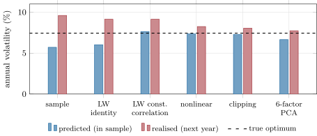
A minimum-variance portfolio of 200 stocks, built from the sample covariance of two years of daily returns, promises an annual volatility of 5.7%. Held for the next year, it runs at 9.6%. Nothing broke, and the market did not change: in the chapter’s simulation the returns of both years come from the same factor covariance, whose true minimum-variance portfolio has a volatility of 7.4%. With 200 assets and 500 days, the sample covariance matrix has 20 100 parameters estimated from 100 000 numbers, and the optimiser finds the directions where its errors make risk look smallest. This chapter is about what a sample covariance matrix is in high dimension: the law its eigenvalues follow when there is nothing but noise, the few eigenvalues that carry information, and the estimators that clean the rest (shrinkage toward a target, eigenvalue by eigenvalue, clipping, and factor structure), judged by the one test that matters for a portfolio: realised risk against promised risk.

22.1 The sample covariance matrix in high dimension

Definition 22.1 (Covariance matrix, sample covariance matrix)

The covariance matrix of a random vector $r \in \R^N$ is $\Sigma = \E[(r - \mu)(r - \mu)^\top]$. From $T$ observations $r_1, \dots, r_T$ with sample mean $\bar r$, the sample covariance matrix is $S = \frac1T\sum_t(r_t - \bar r)(r_t - \bar r)^\top$ (or with divisor $T - 1$).

Definition 22.2 (Principal component analysis, minimum-variance portfolio)

Principal component analysis diagonalises a covariance (or correlation) matrix, $S = U\Lambda U^\top$: the eigenvectors are uncorrelated portfolios and the eigenvalues their variances, in decreasing order. The minimum-variance portfolio for a covariance $\Sigma$ is $w = \Sigma^{-1}\mathbf 1/(\mathbf 1^\top\Sigma^{-1}\mathbf 1)$, the fully invested portfolio of smallest variance, $1/(\mathbf 1^\top\Sigma^{-1}\mathbf 1)$.

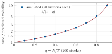
The minimum-variance portfolio needs no expected returns, which makes it the cleanest test of a covariance estimate; it also inverts the matrix, which makes it the harshest. $\Sigma^{-1}$ weights each eigenvector by the reciprocal of its eigenvalue, so the smallest sample eigenvalues, the ones most depressed by noise, get the most weight. With $q = N/T$ held fixed as both grow, and Gaussian returns, the portfolio built from $S$ has an in-sample variance about $(1 - q)$ times the true minimum and a true variance about $1/(1 - q)$ times it: the realised-to-predicted volatility ratio is about $1/(1 - q)$.

The chapter’s truth has 200 stocks, a market factor and five sectors of forty stocks, with specific volatilities between 17% and 44% a year. Over fifty simulated two-year histories ($q = 0.4$), the sample minimum-variance portfolio predicts 5.71% and delivers 9.58% against the truth (9.61% measured over the next 250 days): a ratio of 1.68 against the formula’s $1/(1 - 0.4) = 1.67$. Varying the history from eight years to under one ($q$ from 0.1 to 0.9), the simulated ratio tracks the formula throughout, reaching 10.1 at $q = 0.9$ (Figure 22.1).

22.2 The eigenvalue law of pure noise

Theorem 22.3 (Marchenko–Pastur law)

If the $T \times N$ matrix of returns has iid entries of mean zero and variance $\sigma^2$ and $N/T \to q \in (0, 1)$, the empirical distribution of the eigenvalues of the sample covariance matrix converges to the Marchenko–Pastur law, with density

$$\rho(\lambda) = \frac{\sqrt{(\lambda_+ - \lambda)(\lambda - \lambda_-)}}{2\pi q\sigma^2\lambda}, \qquad \lambda_\pm = \sigma^2(1 \pm \sqrt q)^2,$$

on $[\lambda_-, \lambda_+]$ (Marchenko and Pastur, 1967).

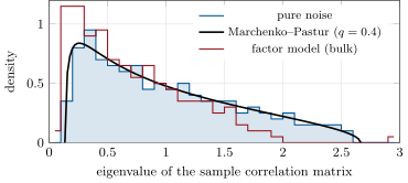
The true eigenvalues are all $\sigma^2$; the sample spreads them from $0.14\sigma^2$ to $2.66\sigma^2$ at $q = 0.4$. The smallest are too small by a factor of seven, and they are the directions a minimum-variance optimiser loves. On 500 days of 200 independent standard normal series, the sample correlation eigenvalues range from 0.144 to 2.565, inside the theoretical edges 0.135 and 2.665 (Figure 22.2); Laloux, Cizeau, Bouchaud and Potters (1999) found most of the eigenvalues of real equity correlation matrices inside the same law.

Definition 22.4 (Spiked covariance model)

In the spiked covariance model (Johnstone, 2001) the population covariance is the identity except for a few eigenvalues $\ell_1, \dots, \ell_k > 1$, the spikes, standing for factors above a noise floor.

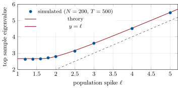
A spike is visible only if it is large enough: when $\ell \le 1 + \sqrt q$ the top sample eigenvalue sticks to the edge $(1 + \sqrt q)^2$; above that threshold it separates and converges to $\ell(1 + q/(\ell - 1))$, larger than $\ell$ (Baik, Ben Arous and Péché, 2005, for complex data; Baik and Silverstein, 2006, for real). At $q = 0.4$ the threshold is 1.63: a factor explaining less than 1.63 times an average stock’s variance is invisible in two years of daily data, however real (Figure 22.3). In the factor model, five sample eigenvalues exceed the edge: the market’s 51.4 (population 52.9) and four sector eigenvalues from 2.96 to 3.68 (population 2.83 to 2.99), each pushed up as the formula says.

22.3 Linear and nonlinear shrinkage

Definition 22.5 (Linear shrinkage)

Linear shrinkage replaces $S$ by $\delta F + (1 - \delta)S$ for a structured target $F$, such as a multiple of the identity or the constant-correlation matrix, with an intensity $\delta \in [0, 1]$ chosen to minimise the expected Frobenius distance to $\Sigma$.

It is chapter 14’s James–Stein idea applied to a matrix. Ledoit and Wolf (2004) derived consistent estimates of the optimal intensity, which needs only the data. Toward $mI$, $m = \operatorname{tr}S/N$, it is $\min(\bar b^2, d^2)/d^2$ with $d^2 = \lVert S - mI\rVert^2/N$ and $\bar b^2 = T^{-2}\sum_t\lVert r_tr_t^\top - S\rVert^2/N$, the dispersion of $S$ around the target against its own sampling noise. On the chapter’s histories the intensity toward the identity averages 0.034 and moves the realised volatility from 9.61% to only 9.14%: the identity is a poor target when stocks share a market factor. Toward constant correlation the intensity is 0.178, the prediction becomes honest (7.64%), but the realised volatility stays at 9.14%.

Definition 22.6 (Rotation-equivariant estimator, nonlinear shrinkage)

A rotation-equivariant estimator keeps the sample eigenvectors and changes only the eigenvalues: $\hat\Sigma = U\operatorname{diag}(d)U^\top$. Nonlinear shrinkage chooses each $d_i$ separately, as an estimate of the oracle value $u_i^\top\Sigma u_i$, the true variance of the $i$-th sample eigenportfolio.

The oracle eigenvalues are the best a rotation-equivariant estimator can do (they minimise the Frobenius error given $U$). They are unknown, but random-matrix theory expresses them through the Stieltjes transform of the limiting eigenvalue density, which can be estimated from the sample eigenvalues themselves; Ledoit and Wolf (2020) gave a closed-form version with a kernel density estimate and its Hilbert transform. On a test with population eigenvalues spread from 0.5 to 2, it cuts the mean squared error of the eigenvalues against the oracle from 0.49 to 0.0034. On the portfolio test it predicts 7.36% and realises 8.25%.

22.4 Eigenvalue clipping and factor structure

Definition 22.7 (Eigenvalue clipping)

Eigenvalue clipping (Laloux et al., 1999) keeps the eigenvalues of the sample correlation matrix above the Marchenko–Pastur edge and replaces all the others by their average, which preserves the trace, then restores the sample variances.

Definition 22.8 (Factor model)

A factor model of covariance is $\Sigma = BF B^\top + D$, with $k \ll N$ factor exposures $B$, a factor covariance $F$ and a diagonal specific variance $D$; statistical factor models take $B$ from the leading principal components of $S$.

Clipping predicts 7.27% and realises 8.05%; a six-factor principal-component model with a diagonal remainder predicts 6.65% and realises 7.74%, closest to the true optimum of 7.44% (Figure 22.4). The ratios of realised to predicted volatility are 1.68 (sample), 1.51 (linear to the identity), 1.19 (linear to constant correlation), 1.12 (nonlinear), 1.11 (clipping) and 1.17 (factor model). The factor model wins here because the truth is a factor model with six factors, which the principal components recover; with a less tidy truth the nonlinear estimator, which assumes nothing about structure, is the safer default. Fan, Liao and Mincheva (2013) combine the two: factors for the spikes, thresholding for the remainder.

22.5 Tutorial: the portfolio that promised 6%

22.6 Build: the covariance estimators

22.7 Exercises

Exercise 22.1 ★

What are the Marchenko–Pastur edges for $N = 500$ stocks and $T = 1\,250$ days?

Solution

Solution of Exercise 22.1.

$q = 0.4$: $\lambda_\pm = (1 \pm \sqrt{0.4})^2 = 0.135$ and $2.665$ (for a correlation matrix, $\sigma^2 = 1$).

Exercise 22.2 ★

A sample minimum-variance portfolio of 300 stocks built from 600 days predicts 5%. What volatility should one expect?

Solution

Solution of Exercise 22.2.

$q = 0.5$, so the true volatility is about $5\%/(1 - 0.5) = 10\%$.

Exercise 22.3 ★

Show that the minimum-variance portfolio’s variance is $1/(\mathbf 1^\top\Sigma^{-1}\mathbf 1)$.

Solution

Solution of Exercise 22.3.

With $w = \Sigma^{-1}\mathbf 1/c$, $c = \mathbf 1^\top\Sigma^{-1}\mathbf 1$: $w^\top\Sigma w = \mathbf 1^\top\Sigma^{-1}\Sigma\Sigma^{-1}\mathbf 1/c^2 = c/c^2 = 1/c$.

Exercise 22.4 ★★

With $q = 0.25$, which population spikes are detectable, and where does a spike of 3 appear in the sample?

Solution

Solution of Exercise 22.4.

Spikes above $1 + \sqrt{0.25} = 1.5$. A spike of 3 appears at $3(1 + 0.25/2) = 3.375$, above the edge $(1.5)^2 = 2.25$.

Exercise 22.5 ★★

Show that the linear shrinkage $\delta mI + (1 - \delta)S$ keeps the eigenvectors of $S$ and maps each eigenvalue $\lambda$ to $\delta m + (1 - \delta)\lambda$. Why is this less flexible than nonlinear shrinkage?

Solution

Solution of Exercise 22.5.

$\delta mI + (1 - \delta)U\Lambda U^\top = U(\delta mI + (1 - \delta)\Lambda)U^\top$. Every eigenvalue is pulled toward $m$ by the same fraction, so the small eigenvalues, which are too small, and the large ones, which are too large, are corrected by one number; the oracle correction is not linear in $\lambda$, and nonlinear shrinkage chooses it eigenvalue by eigenvalue.

Exercise 22.6 ★★

How many days of data would make the sample minimum-variance portfolio of 200 stocks underpredict its volatility by at most 10%?

Solution

Solution of Exercise 22.6.

$1/(1 - q) \le 1.1$ requires $q \le 0.091$, so $T \ge 200/0.091 = 2\,200$ days, about 8.7 years; over such a span the covariance itself changes.

Exercise 22.7 ★★★

Coding. Reproduce the ratio of true to predicted volatility of the sample minimum-variance portfolio for $q$ from 0.1 to 0.9 and compare it with $1/(1 - q)$.

Solution

Solution of Exercise 22.7.

bias_vs_q(): 1.11, 1.26, 1.43, 1.67, 2.05, 2.51, 3.38, 5.21 and 10.05 at $q = 0.1$ to 0.9, against 1.11, 1.25, 1.43, 1.67, 2.00, 2.50, 3.33, 5.00 and 10.09.

Exercise 22.8 ★★★

Find the flaw. “We chose our covariance estimator because it has the lowest in-sample minimum-variance portfolio volatility of all the estimators we tried.”

Solution

Solution of Exercise 22.8.

The in-sample volatility of a minimum-variance portfolio is lowest for the estimator whose small eigenvalues are most underestimated, that is the noisiest: in the chapter the raw sample covariance has the lowest in-sample figure (5.7%) and the worst realised risk (9.6%). Select estimators by out-of-sample risk, or by the realised-to-predicted ratio.

22.8 Problem: The Portfolio That Promised 6%

Problem 22.1

Weekend problem — risk promised and risk delivered

Two hundred stocks follow a known covariance with a market factor and five sectors of forty. A manager estimates the covariance from two years (500 days) of daily returns, builds the minimum-variance portfolio and holds it for a year. Fifty histories are simulated.

Part I — The sample.

1. What does the sample portfolio predict and deliver, and what is the true optimum?
2. What ratio does the formula $1/(1 - q)$ predict, and what does the simulation give?
3. What are the Marchenko–Pastur edges at $q = 0.4$, and where do pure-noise eigenvalues fall?
4. Which eigenvalues of the factor model stand out, and by how much are they biased?
5. What is the smallest detectable factor at this $q$?

Part II — Better estimators.

6. What intensities do the two linear shrinkages choose, and what do they deliver?
7. What do nonlinear shrinkage and clipping deliver?
8. What does the six-factor model deliver, and why is it best here?
9. What are the realised-to-predicted ratios of all six?
10. Which estimator’s prediction is most honest, and which portfolio is best?

Part III — Dimensions.

11. What happens to the sample portfolio at $q = 0.9$?
12. How many days would make the ratio 1.1?
13. Why does the optimiser pick the noisiest directions?
14. What does a long-only constraint do to this problem?
15. Why does the identity make a poor shrinkage target for stocks?

Part IV — Judgement.

16. Which estimator would you put in production, and why?
17. How would you monitor it?
18. What would change with fat-tailed returns or a changing covariance?
19. State the named result: the realised-to-predicted risk ratio of the sample portfolio at $q = 0.4$ against $1/(1 - q)$, and the ratio each better estimator achieves.
20. In one sentence: why does an optimiser make estimation error worse?

Solution

Solution of Problem 22.1.

1. Predicts 5.71%, delivers 9.58% against the truth (9.61% over the next year); the true optimum is 7.44%. 2. $1/(1 - 0.4) = 1.67$; the simulation gives 1.68. 3. 0.135 and 2.665; on pure noise the sample eigenvalues run from 0.144 to 2.565. 4. The market (51.4 against 52.9 in the population) and four sectors (2.96 to 3.68 against 2.83 to 2.99): the sector eigenvalues are pushed up by the noise, as $\ell(1 + q/(\ell - 1))$ predicts. 5. A spike of $1 + \sqrt{0.4} = 1.63$ times the noise variance. 6. 0.034 toward the identity, delivering 9.14%; 0.178 toward constant correlation, also 9.14% but with an honest prediction (7.64%). 7. Nonlinear shrinkage 8.25% (predicts 7.36%); clipping 8.05% (predicts 7.27%). 8. 7.74% (predicts 6.65%): the truth is a six-factor model, which six principal components recover, and the diagonal remainder is exactly right. 9. 1.68, 1.51, 1.19, 1.12, 1.11 and 1.17. 10. Clipping and nonlinear shrinkage have the most honest predictions (ratios 1.11 and 1.12); the factor model builds the best portfolio (7.74%). 11. Its true volatility is ten times its prediction (10.05 simulated, 10.09 by the formula). 12. $q \le 0.091$: 2 200 days. 13. It weights each direction by the inverse of its estimated variance, and the most underestimated variances are noise; the optimiser concentrates exactly where the estimate is worst. 14. It forbids the large offsetting positions that exploit noise, which acts as a form of shrinkage (at the cost of excluding genuinely useful shorts). 15. Stocks share a market factor; the identity target says they are uncorrelated, so a strong shrinkage toward it would be badly wrong and the optimal intensity stays tiny (0.034). 16. Nonlinear shrinkage or a factor model with a shrunk remainder, cross-checked by clipping; not the raw sample. 17. Track realised against predicted volatility of the production portfolios on a rolling window, and the stability of the eigenvalues above the edge. 18. Heavier tails widen the eigenvalue spread and favour robust or rank-based estimates; a changing covariance shortens the usable history, which raises $q$ and makes cleaning more important. 19. Named result: the portfolio that promised 6%: at $q = 0.4$ the sample minimum-variance portfolio delivers 1.68 times the volatility it predicts (5.71% promised, 9.58% delivered), against $1/(1 - q) = 1.67$; linear shrinkage toward the identity gives 1.51, toward constant correlation 1.19, nonlinear shrinkage 1.12, clipping 1.11 and a six-factor model 1.17. 20. Because it seeks the directions of smallest estimated risk, which are the directions where estimation error has made risk look smallest.

22.9 Interview questions

Interview question 22.1 ★ researcher, risk

Why does a minimum-variance portfolio built from a sample covariance underpredict its risk?

Solution

Solution of Interview question 22.1.

The optimiser selects the directions whose sample variance is smallest, and those are, disproportionately, directions where noise has pushed the estimate down; in high dimension the in-sample variance is biased down by about $1 - q$ and the true variance up by $1/(1 - q)$, $q = N/T$.

What the interviewer is looking for: Selection on noise and the $1/(1 - q)$ scaling.

Interview question 22.2 ★★ researcher, mle

What is the Marchenko–Pastur law, and how do you use it on a correlation matrix?

Solution

Solution of Interview question 22.2.

The limiting eigenvalue density of a sample covariance of pure noise, supported on $[\sigma^2(1 - \sqrt q)^2, \sigma^2(1 + \sqrt q)^2]$. On a correlation matrix, eigenvalues above the upper edge carry information (market, sectors); those inside the bulk are indistinguishable from noise and can be cleaned (clipped or shrunk).

What the interviewer is looking for: The edges, and the bulk-versus-spikes reading.

Interview question 22.3 ★★ researcher

Explain Ledoit–Wolf shrinkage. What does the intensity depend on?

Solution

Solution of Interview question 22.3.

A convex combination of the sample covariance and a structured target, with the intensity that minimises the expected Frobenius loss, estimated from the data. The intensity grows with the sampling noise of $S$ (large $N/T$, fat tails) and shrinks with the distance between $S$ and the target.

What the interviewer is looking for: Bias-variance trade and what drives the intensity.

Interview question 22.4 ★★ researcher, risk

You have 1 000 stocks and three years of daily data. How do you estimate the covariance matrix?

Solution

Solution of Interview question 22.4.

$q = 1\,000/750 > 1$: the sample covariance is singular. Use a factor model (statistical or fundamental) for the common part with a diagonal or shrunk remainder, or nonlinear shrinkage designed for $N > T$; check by the realised risk of the portfolios it produces.

What the interviewer is looking for: Recognising singularity and using structure.

Interview question 22.5 ★★ mle, researcher

How many principal components of a stock correlation matrix carry information?

Solution

Solution of Interview question 22.5.

Those whose eigenvalues exceed the Marchenko–Pastur upper edge for the sample’s $q$ (after accounting for the variance they take from the bulk): typically the market and a handful of sectors; the rest cannot be told from noise with that much data.

What the interviewer is looking for: The edge as the criterion, and the spike threshold.

Interview question 22.6 ★★★ researcher

What is a rotation-equivariant estimator, and what is the best one could do in that class?

Solution

Solution of Interview question 22.6.

An estimator that keeps the sample eigenvectors and changes only the eigenvalues, so it transforms consistently with any rotation of the data. The best in the class uses the oracle eigenvalues $u_i^\top\Sigma u_i$, the true variance of each sample eigenportfolio; nonlinear shrinkage estimates them from the sample spectrum through random-matrix theory.

What the interviewer is looking for: Equivariance, the oracle, and how it is approximated.