8Markov Chains and Queues

At the best bid of a large-tick future sit 800 lots; at the best ask, 200. A market maker has just joined the back of the bid queue and wants to know two things: how likely its order is to be filled before the ask queue is eaten and the price ticks up, leaving the order stranded; and how long it will wait. Both are questions about the time a random walk takes to hit zero. If orders join and leave a queue at random times, each queue is a Markov chain, and the answers follow from the chain’s generator: 73% and 82 seconds, for the rates of this chapter, against 99% if the ask queue were twice as long. This chapter sets out continuous-time Markov chains, the birth–death processes and simple queues built from them, the first-step analysis that computes hitting probabilities and times, and a model of the two best queues of an order book in the spirit of Cont and de Larrard (2013).

8.1 Continuous-time Markov chains

Definition 8.1 (Markov chain, continuous-time Markov chain)

A Markov chain is a Markov process with a countable state space, observed at integer times, with transition matrix $P_{ij} = \P(X_{n+1} = j \mid X_n = i)$. A continuous-time Markov chain is a right-continuous Markov process $(X_t)_{t\ge0}$ with a countable state space whose transition probabilities $P_{ij}(t) = \P(X_{s+t} = j \mid X_s = i)$ do not depend on $s$.

Definition 8.2 (Generator matrix, jump chain)

The generator matrix of a continuous-time chain is $\mathcal L = (q_{ij})$ with $q_{ij} = \lim_{t\downarrow0}P_{ij}(t)/t \ge 0$ for $j \ne i$, the rate of jumps from $i$ to $j$, and $q_{ii} = -\sum_{j\ne i}q_{ij}$. The jump chain is the discrete-time chain of the states visited, with transition probabilities $q_{ij}/q_i$, where $q_i = -q_{ii}$.

Proposition 8.3 (Construction and Kolmogorov equations)

A finite chain with generator $\mathcal L$ stays in state $i$ for an exponential time with rate $q_i$, then moves according to the jump chain, independently of the past. Its transition matrix is $P(t) = e^{t\mathcal L}$, which solves $P'(t) = P(t)\mathcal L = \mathcal LP(t)$, the forward and backward equations.

A continuous-time chain is the discrete generator of chapter 4 for a finite state space: the same backward and forward equations, with a matrix instead of a differential operator. Its stationary distribution solves $\pi\mathcal L = 0$.

Example 8.4 (The spread in ticks)

Model a large-tick contract’s spread as 1, 2 or 3 ticks, widening from 1 to 2 at rate 2 per second and from 2 to 3 at rate 1, narrowing from 2 to 1 at rate 5, from 3 to 2 at rate 4 and from 3 to 1 at rate 0.5. Solving $\pi\mathcal L = 0$ gives $\pi = (0.676, 0.265, 0.059)$, a mean spread of 1.38 ticks; the spread sits at one tick for 0.5 seconds on average before widening.

Definition 8.5 (Detailed balance)

A distribution $\pi$ satisfies detailed balance with a generator if $\pi_iq_{ij} = \pi_jq_{ji}$ for all $i, j$: in stationarity every transition is as frequent as its reverse, and the chain run backwards in time has the same law (it is reversible).

Detailed balance implies $\pi\mathcal L = 0$ by summing over $i$; the converse fails when probability circulates around a cycle, as it does in the spread example (Exercise 8.4). Birth–death chains, which move one step at a time, always satisfy it.

8.2 Birth–death processes and simple queues

Definition 8.6 (Birth–death process)

A birth–death process is a continuous-time chain on $\{0, 1, 2, \dots\}$ whose only jumps are $n \to n + 1$ at rate $\lambda_n$ and $n \to n - 1$ at rate $\mu_n$.

Proposition 8.7 (Stationary law of a birth–death process)

If $\sum_n\prod_{k=1}^n\lambda_{k-1}/\mu_k < \infty$, the stationary law is $\pi_n \propto \prod_{k=1}^n\lambda_{k-1}/\mu_k$.

Definition 8.8 (M/M/1 queue)

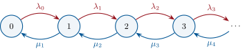
The M/M/1 queue has Poisson arrivals at rate $\lambda$, exponential service times with rate $\mu$ and one server; the number in the system is a birth–death process with $\lambda_n = \lambda$ and $\mu_n = \mu$. (Kendall’s notation: Markov arrivals, Markov service, one server.)

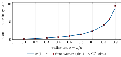
With utilisation $\rho = \lambda/\mu < 1$ the stationary law is geometric, $\pi_n = (1 - \rho)\rho^n$, so the mean number in the system is $L = \rho/(1 - \rho)$. Little’s law, $L = \lambda W$ for the mean time $W$ spent in the system, holds for almost any stationary queue (Little, 1961), and gives $W = 1/(\mu - \lambda)$. Both explode as $\rho \to 1$: a matching engine or a risk gate that runs at 90% of its capacity has nine messages waiting on average, at 95% nineteen (Figure 8.2). One Quant Book 13 sizes its queues with these formulas.

8.3 Hitting probabilities and hitting times

Definition 8.9 (Absorbing state, hitting probability)

A state is an absorbing state if the chain never leaves it ($q_i = 0$). For a set $A$ of states, the hitting probability $h_i = \P_i(\text{the chain ever enters } A)$.

Method 8.10 (First-step analysis)

First-step analysis conditions on the first jump. Hitting probabilities solve $h_i = 1$ on $A$ and $\sum_jq_{ij}h_j = 0$ off $A$; expected hitting times $m_i$ solve $m_i = 0$ on $A$ and $\sum_jq_{ij}m_j = -1$ off $A$ (the minimal nonnegative solutions). For a birth–death chain these systems are tridiagonal and cost $O(n)$ to solve.

For a queue with constant rates $\lambda$ and $\mu$, the probability of reaching $n$ before 0 from $i$ is the gambler’s ruin of chapter 1, $(1 - (\mu/\lambda)^i)/(1 - (\mu/\lambda)^n)$, and the expected time to empty from $i$ when $\mu > \lambda$ is $i/(\mu - \lambda)$. Means hide a lot here: the law of the emptying time is skewed, and a race between two queues needs the whole law. It comes from uniformisation: with $L$ at least every total rate, the chain is a jump chain with transition matrix $I + \mathcal L/L$ run at the times of a Poisson process of rate $L$, so $P(t) = \sum_k e^{-Lt}\frac{(Lt)^k}{k!}(I + \mathcal L/L)^k$, a sum of positive terms that is stable to compute (tutorial, first listing).

8.4 Queues sized for order books

Count each best queue in orders of 10 lots. On each side, limit orders join at rate $\lambda = 0.9$ per second, and orders leave, by market orders ($0.6$) and cancellations ($0.4$), at rate $\nu = 1$: the queues drift toward zero, and when one empties the price moves. Take the two queues independent. Then the mid price moves up next if the ask queue’s emptying time $T_a$ comes before the bid’s, and

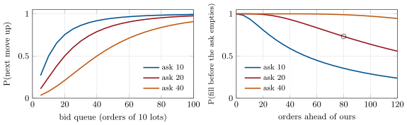
with $F_a, F_b$ the laws of the emptying times. Figure 8.3 shows it against the queue sizes: with 800 lots bid and 200 offered, the next move is up with probability 95.4%. Queue imbalance predicts the next tick, a fact One Quant Book 10 turns into a signal.

For the market maker’s order at the back of the bid, with $k$ orders ahead, the fill time is the time for the $k$ orders ahead to leave (at rate $\nu$ each) plus the wait for a market order (rate $0.6$), independent of the ask queue. The fill probability is the race of that time against $T_a$ (Figure 8.3). With 80 orders ahead and 20 on the ask, it is 73.2%, and 73.4% in 20 000 simulated races; with 20 ahead it would be 99.3%. A place near the front of the queue is worth money, which is why time priority is contested so hard (One Quant Book 1, chapter 19).

8.5 Tutorial: the back of the queue

8.6 Build: queues for order books

8.7 Exercises

Exercise 8.1 ★

In the spread chain of Example 8.4, what is the mean time spent at each spread before a change, and where does the chain go when it leaves 3 ticks?

Solution

Solution of Exercise 8.1.

Mean holding times $1/q_i$: 0.5 s at one tick, $1/6$ s at two, $2/9 = 0.22$ s at three. From three ticks the chain goes to two with probability $4/4.5 = 0.889$ and to one with $0.111$.

Exercise 8.2 ★

An M/M/1 queue serves one message a microsecond and receives 0.8 a microsecond. What are the mean number of messages in the system and the mean time a message spends there?

Solution

Solution of Exercise 8.2.

$\rho = 0.8$: $L = 0.8/0.2 = 4$ messages, $W = 1/(1 - 0.8) = 5$ microseconds, and $L = \lambda W$.

Exercise 8.3 ★

A queue of 20 orders gains one at rate 0.9 and loses one at rate 1. What is the probability it reaches 40 before emptying?

Solution

Solution of Exercise 8.3.

$(1 - (1/0.9)^{20})/(1 - (1/0.9)^{40}) = 10.8\%$.

Exercise 8.4 ★★

Is the spread chain reversible? Check detailed balance between 1 and 2 ticks, and Kolmogorov’s criterion on the cycle $1 \to 2 \to 3 \to 1$.

Solution

Solution of Exercise 8.4.

No. $\pi_1q_{12} = 0.676 \times 2 = 1.35$ but $\pi_2q_{21} = 0.265 \times 5 = 1.32$: detailed balance fails. Kolmogorov’s criterion compares $q_{12}q_{23}q_{31} = 2 \times 1 \times 0.5 = 1$ with $q_{13}q_{32}q_{21} = 0$: probability circulates $1 \to 2 \to 3 \to 1$.

Exercise 8.5 ★★

For the queue of Exercise 8.3 with no upper limit, what are the mean and the median time to empty, and the probability it empties within a minute? Why do mean and median differ so much?

Solution

Solution of Exercise 8.5.

Mean $20/(1 - 0.9) = 200$ s, median 137 s, and 15.6% within a minute. The law is skewed to the right: most paths empty sooner than average, a few wander far up first and take very long.

Exercise 8.6 ★★

A price level holds 400 lots on average, and 50 lots a second leave it by execution or cancellation. How long does a lot rest there on average?

Solution

Solution of Exercise 8.6.

By Little’s law $W = L/\lambda = 400/50 = 8$ seconds.

Exercise 8.7 ★★★

Coding. Check the fill probability of the weekend problem by simulating the race event by event, and compare with the uniformisation result.

Solution

Solution of Exercise 8.7.

73.4% in 20 000 seeded races, against 73.2% by uniformisation: within the simulation’s standard error of 0.3 point.

Exercise 8.8 ★★★

Find the flaw. “Our passive orders get filled 95% of the time when the book is this imbalanced, so we join the back of the heavy side whenever we see it.”

Solution

Solution of Exercise 8.8.

The 95% is the probability that the next tick is up, not a fill rate: an order at the back of the heavy bid fills before the thin ask empties only 73% of the time, and less if it is further back. And fills are not a random sample: an order at the bid fills when sellers keep hitting it, often just before the price moves down. The decision needs the mark-out after fills, not the fill rate.

8.8 Problem: The Back of the Queue

Problem 8.1

Weekend problem — 800 lots ahead, 200 on the other side

A market maker’s order joins the back of a best bid of 800 lots; the best ask holds 200. Orders are 10 lots. On each side limit orders join at 0.9 per second, market orders arrive at 0.6 per second and cancellations at 0.4, so orders leave at $\nu = 1$ per second. Take the queues independent.

Part I — The model.

1. How many orders are ahead of ours, and on the ask?
2. What is the expected time until our order is filled, ignoring the ask?
3. What are the mean and the median time for the ask queue to empty?
4. What is the probability that the ask empties within a minute?
5. What is the probability that it empties at all?

Part II — The race.

6. What is the probability that our order fills before the ask empties?
7. What does a simulation of 20 000 races give?
8. And if the ask held 400 or 800 lots?
9. And if only 20 orders were ahead of ours?
10. What is the probability that the next move of the mid is up, and with equal queues?

Part III — First steps.

11. What is the probability that the ask queue reaches 40 orders before it empties?
12. What is the expected time until it first reaches 0 or 40?
13. How would cancellations proportional to the queue size change the drift?
14. What would clustered order flow (chapter 7) do to the tail of the emptying time?
15. What does independence of the two queues leave out?

Part IV — Judgement.

16. What is a queue position worth, in this model?
17. When the order does fill in this configuration, what does the fill tell the market maker?
18. Should it join the bid at all?
19. State the named result: the fill probability and the expected wait.
20. In one sentence: what decides whether a passive order at the back of a queue fills?

Solution

Solution of Problem 8.1.

1. 80 orders ahead; 20 on the ask. 2. $80/1 + 1/0.6 = 81.7$ seconds. 3. Mean $20/(1 - 0.9) = 200$ s; median 137 s. 4. 15.6%. 5. One: the queue drifts down at 0.1 order a second (99.6% of paths within 20 minutes). 6. 73.2%. 7. 73.4%. 8. 99.0% with 40 orders on the ask; with 80, the ask practically never empties first. 9. 99.3%. 10. 95.4% up with 80 against 20; 50% with equal queues. 11. 10.8%. 12. 156.6 seconds. 13. Departures would grow with the queue, pulling long queues down and short ones up: a mean-reverting size instead of a constant drift, and fewer extreme queues. 14. Bursts make some queues empty much faster and others last longer: fatter tails on both sides, and a fill probability that depends on the state of the flow. 15. The dependence between the sides: a large buy empties the ask and brings in new bids, and liquidity providers react to imbalance (the queue-reactive models of One Quant Book 10). 16. The difference in fill probability between the front and the back, $100\%$ against $73\%$ here, times the value of a fill (half the spread less the expected adverse move). 17. That the bid was hit 80 times before the ask emptied: sellers were aggressive, and the price is more likely to fall next than the unconditional numbers say. 18. Only if half the spread exceeds the expected adverse move after a fill (the mark-out, One Quant Book 2, chapter 15); the model gives the fill probability, not the answer. 19. Named result: the back of the queue: with 80 orders ahead and 20 on the ask, the order fills before the ask empties with probability 73% (73.2% exact, 73.4% simulated), after 82 seconds on average; with the ask twice as long, 99%. 20. The race between the orders ahead leaving and the other side’s queue emptying.

8.9 Interview questions

Interview question 8.1 ★ researcher, developer

A server handles 10 000 requests a second and receives 9 000. On average, how many are waiting and for how long?

Solution

Solution of Interview question 8.1.

As an M/M/1 queue with $\rho = 0.9$: 9 requests in the system on average (8.1 waiting), each spending $1/(10\,000 - 9\,000)$ s $= 1$ ms, ten times the service time.

What the interviewer is looking for: $\rho/(1-\rho)$ and Little’s law, and the blow-up near saturation.

Interview question 8.2 ★ researcher

What is the generator of a continuous-time Markov chain, and how do you get its stationary distribution?

Solution

Solution of Interview question 8.2.

The matrix of jump rates $q_{ij}$, with diagonal minus the row sums; $P(t) = e^{t\mathcal L}$. The stationary distribution solves $\pi\mathcal L = 0$ with $\sum\pi_i = 1$; for a birth–death chain, detailed balance gives it in closed form.

What the interviewer is looking for: rates, holding times, and $\pi\mathcal L = 0$.

Interview question 8.3 ★★ trader, researcher

The bid has 800 lots and the ask 200. Which way is the next tick more likely, and why?

Solution

Solution of Interview question 8.3.

Up: the thin ask empties sooner than the heavy bid, and the first queue to empty moves the price. With the chapter’s rates, 95%.

What the interviewer is looking for: queue depletion as a race.

Interview question 8.4 ★★ researcher

A fair random walk starts at 3. What are the probability of hitting 10 before 0 and the expected number of steps?

Solution

Solution of Interview question 8.4.

$3/10$, by optional stopping; the expected number of steps is $3 \times 7 = 21$, from $W_n^2 - n$.

What the interviewer is looking for: gambler’s ruin and $i(n - i)$.

Interview question 8.5 ★★ trader

Why do market makers value a place at the front of the queue, and how would you put a number on it?

Solution

Solution of Interview question 8.5.

The front fills first and more often, before the price moves away, and the back fills mainly when the queue is being eaten by informed flow. Value it as the difference in fill probability times the edge per fill, with fill probabilities from a queue model or from the firm’s own fill data by queue position.

What the interviewer is looking for: fill probability by position, and adverse selection.

Interview question 8.6 ★★★ developer, researcher

How do you compute the probability that a chain is in a given state after time $t$, for a chain with thousands of states, stably?

Solution

Solution of Interview question 8.6.

Uniformisation: pick $L$ at least every exit rate, run the jump matrix $I + \mathcal L/L$ on a vector (sparse matrix–vector products) and weight the iterates by Poisson probabilities. Every term is nonnegative, so there is no cancellation, unlike a Taylor series of $e^{t\mathcal L}$.

What the interviewer is looking for: uniformisation, sparsity, and positivity.