University Biology — Year 1 · Bachelor Year 1

25Populations and Demography

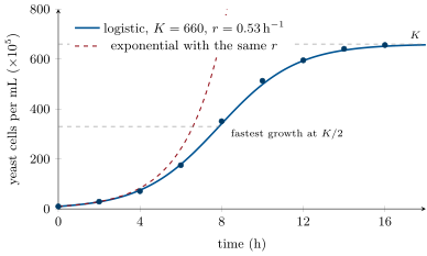
A flask of yeast starts with a million cells and, sixteen hours later, holds sixty million and has stopped growing; a herd of deer on an island grows by a tenth each year until the winter its food runs out; the lynx of the boreal forest rise and crash every ten years, a year behind the hares they eat. Each is a population — the individuals of one species in one place — and each obeys arithmetic that can be written down. This chapter describes how populations are counted, how their births and deaths are tabulated, the two equations of growth, the forces that hold numbers in check, and what the same arithmetic says about our own species.

25.1 Counting a population

Definition 25.1 (Population, density, dispersion)

A population is the set of individuals of one species living in a given area at a given time and able to interbreed. Its size $N$ is the number of individuals; its density the number per unit area or volume; its dispersion the pattern of their spacing — clumped where resources or social life gather them (herds, schools, patches of a plant), uniform where they repel one another (territorial birds, desert shrubs competing for water), random where neither operates. Populations also have an age structure, a sex ratio, and rates of birth, death, immigration and emigration, whose balance is the growth.

Method 25.2 (Estimating a population)

Sessile or slow organisms: count in quadrats of known area placed at random, and multiply the mean density by the total area; the scatter among quadrats gives the precision and reveals the dispersion.
Mobile animals: mark–recapture. Catch $M$ individuals, mark and release them; later catch $C$ , of which $R$ are marked. If the marked mix freely and nothing has changed, the marked fraction of the second catch equals the marked fraction of the population, $R/C = M/N$ , so $N \approx MC/R$ (the Lincoln–Petersen estimate).
Check the assumptions: no births, deaths or migration between the catches, marks that neither fall off nor change the animal’s behaviour, equal catchability. Each failure biases $N$ in a predictable direction.
Indirect signs where counting is impossible: droppings, tracks, calls, nests, the DNA in a litre of pond water.

Example 25.3 (Voles in a meadow)

Sixty voles trapped, marked and released in a hectare of meadow; three nights later eighty are trapped, of which twelve carry marks: $N \approx 60\times 80/12 = 400$ voles, four per hundred square metres. If the marked voles, having learned that traps hold food, are caught more readily, $R$ is inflated and $N$ underestimated; if marking frightened them away from traps, the reverse.

25.2 Demography: births and deaths by age

Definition 25.4 (Life table)

A life table follows a cohort of individuals born together through their lives. For each age $x$ it records $l_x$ , the survivorship — the fraction of the cohort still alive at age $x$ — and $m_x$ , the fecundity — the mean number of daughters born to a female of age $x$ . From them: the mortality between ages, $q_x = 1 - l_{x+1}/l_x$ ; the net reproductive rate $R_0 = \sum_x l_x m_x$ , the number of daughters a newborn female will have on average in her lifetime; and the generation time $T = \sum_x x\,l_x m_x / R_0$ , the mean age of the mothers of those daughters. A population with $R_0 > 1$ grows, with $R_0 < 1$ declines; over one generation it is multiplied by $R_0$ .

Proposition 25.5 (Three shapes of survivorship)

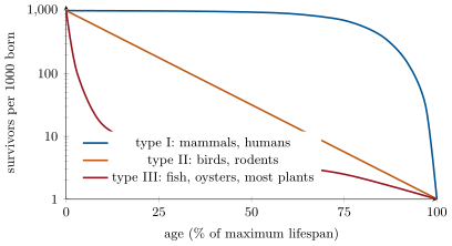
Plotting $\log l_x$ against age gives three types of curve. Type I: most individuals survive to old age and die within a narrow span (large mammals, humans in rich countries). Type II: a constant probability of death at every age, a straight line on the log scale (many birds, lizards, rodents). Type III: enormous mortality among the young and long life for the few survivors (oysters, fish, most plants and insects). The shape follows from the organism’s way of life: a species that invests little in each of many offspring has a type III curve; one that invests much in each of a few, type I.

Three types of survivorship curve, on a logarithmic scale. Type I dies late, type III dies early, type II dies at a constant rate; each is a life history written as a line.

Age pyramids: the number of individuals in each age class, males to the left, females to the right. A broad base means many young and growth to come; even classes mean replacement; a narrow base means decline.

Example 25.6 (A life table for a deer herd)

Of a thousand fawns, six hundred reach their first birthday, and the survivors then lose a tenth of their number each year until few pass nine; does bear from age two, about eight tenths of a daughter a year in their prime. Summing $l_x m_x$ gives $R_0 \approx 1.5$ : each doe leaves one and a half daughters, and the herd grows by half each generation of about four years — an eleven percent increase per year until something stops it.

25.3 Growth

Theorem 25.7 (Exponential growth)

A population whose per-capita birth and death rates $b$ and $d$ are constant grows at a rate proportional to its size,

\frac{\dd N}{\dd t} = rN, \qquad r = b - d, \qquad N(t) = N_0\,e^{rt},

where $r$ is the intrinsic rate of increase. It doubles every $\ln 2/r$ ; a population with $r = 0.11\,\mathrm{yr}^{-1}$ doubles in $6.3\,\mathrm{yr}$ , one with $r = 0.5\,\mathrm{h}^{-1}$ in $83\,\mathrm{min}$ . From a life table, $r \approx \ln R_0 / T$ .

Proof. In a short interval $\dd t$ the births are $bN\,\dd t$ and the deaths $dN\,\dd t$ , so $\dd N = (b - d)N\,\dd t$ ; the equation $\dd N/\dd t = rN$ has the solution $N_0 e^{rt}$ (the derivative of $e^{rt}$ is $re^{rt}$ ). Doubling: $e^{rt} = 2$ gives $t = \ln 2/r$ . Over one generation $T$ the population is multiplied by $R_0 = e^{rT}$ , whence $r = \ln R_0/T$ . ∎

Theorem 25.8 (Logistic growth)

If the per-capita growth rate falls linearly as the population approaches a carrying capacity $K$ — the size the environment can sustain —

\frac{\dd N}{\dd t} = rN\left(1 - \frac{N}{K}\right), \qquad N(t) = \frac{K}{1 + \dfrac{K - N_0}{N_0}\,e^{-rt}} .

Growth is nearly exponential while $N \ll K$ , fastest at $N = K/2$ (where $\dd N/\dd t = rK/4$ ), and vanishes at $N = K$ , which the population approaches as a plateau: an S-shaped curve.

Proof. Write the equation as $\dd N/[N(1 - N/K)] = r\,\dd t$ and split the left side into $\dd N/N + \dd N/(K - N)$ ; integrating gives $\ln[N/(K - N)] = rt + \text{const}$ , and solving for $N$ with $N(0) = N_0$ gives the formula. Differentiating $rN(1 - N/K)$ with respect to $N$ and setting it to zero gives the maximum at $N = K/2$ . ∎

A yeast culture counted every two hours (points), the logistic curve fitted to it, and the exponential it would have followed with no limit. The two agree for the first six hours and then part.

Proposition 25.9 (Density dependence)

Growth slows as density rises because the per-capita birth rate falls or the death rate rises with crowding: food per head declines, territories become unavailable, wastes and disease accumulate, predators concentrate. These density-dependent factors regulate a population toward $K$ . Density-independent factors — frost, flood, fire, drought — kill a fraction regardless of numbers and cannot regulate, only disturb; the populations of many insects are governed mostly by the weather and never approach a carrying capacity.

Evidence. Gause (1934) grew Paramecium in tubes of medium renewed daily: the counts followed a logistic curve to a plateau set by the food, and doubling the food doubled the plateau. Pearl (1927) found the same in fruit flies in bottles, and Carlson (1913) in yeast. In the field, song sparrows on an island lay smaller clutches and lose more young when the breeding population is large, and the number of territories caps the number of breeders; removing birds is followed by their replacement from a surplus that had been excluded. ∎

Definition 25.10 (Life-history strategies)

Species differ in where they sit between two extremes. A $r$ -selected species — weeds, aphids, mice, most fish — is built for a high $r$ : it matures early, produces many small offspring, invests little in each, lives briefly, and exploits new or disturbed habitats before the competition arrives, with a type III survivorship. A $K$ -selected species — oaks, elephants, albatrosses — is built to persist near $K$ : it matures late, produces few large offspring, cares for them, lives long, competes well in crowded stable habitats, with a type I curve. Most species mix the two; the labels name the ends of the scale.

25.4 Fluctuation and regulation

Proposition 25.11 (Cycles of predator and prey)

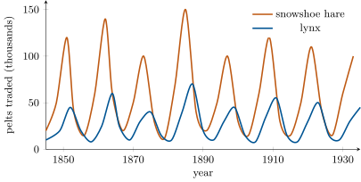
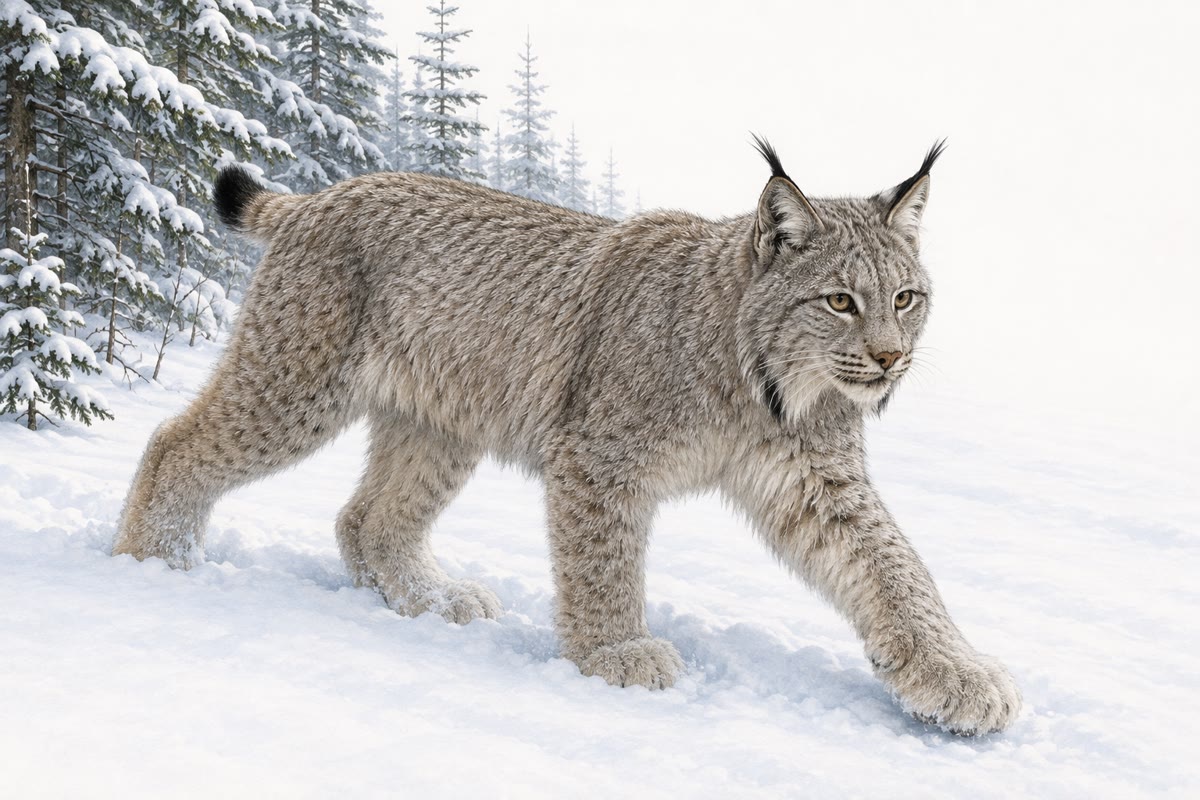
Some populations do not settle but oscillate. The snowshoe hare of the northern forest and the lynx that eats it rise and fall together with a period of about ten years, the lynx a year or two behind the hare: many hares feed many lynx, many lynx eat the hares down, few hares starve the lynx, few lynx let the hares recover. The cycle is driven partly by the predator and partly by the hares’ own food, whose recovery after overbrowsing takes years; models of coupled predator and prey (Chapter 27) reproduce such oscillations from two equations.

Evidence. The fur returns of a trading company, kept for ninety years from the 1840s, record the number of lynx and hare pelts brought in each year across a subcontinent: both series show peaks every nine to ten years, the lynx peak lagging the hare’s, over nine full cycles. Field studies since, with hares fenced from predators or given extra food, show that removing either factor damps the cycle and removing both abolishes it. ∎

Hare and lynx pelts brought to the trading posts of the northern forest, year by year (smoothed). Both cycle with a period of about ten years, the lynx a year or two behind the hare.

A lynx in the boreal forest. Its numbers follow the hare’s with a lag: the predator’s cycle is the prey’s, delayed.

Example 25.12 (Our own species)

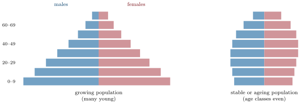
The human population took all of history to reach one billion, in about 1800, and two centuries to reach eight. Its growth rate peaked near $2\,\%$ a year in the 1960s (doubling in 35 years) and has since fallen below $1\,\%$ , not through deaths but through births: where child mortality falls and women are educated, families shrink within a generation, and the age pyramid turns from a triangle to a column. The arithmetic of $R_0$ applies to us; what changed is $m_x$ .

25.5 Exercises

Exercise 25.1 ★

Define population, density and dispersion, and give an example of each pattern of dispersion.

Solution

Solution of Exercise 25.1.

Population: the individuals of one species in one place and time, able to interbreed. Density: individuals per unit area or volume. Dispersion: their spatial pattern — clumped (a herd, a patch of nettles), uniform (nesting gannets a peck apart, creosote bushes), random (dandelions on a lawn).

Exercise 25.2 ★

Define $l_x$ , $m_x$ , $R_0$ and $T$ , and say what $R_0 = 1$ means.

Solution

Solution of Exercise 25.2.

$l_x$ : fraction of a cohort alive at age $x$ . $m_x$ : daughters per female of age $x$ . $R_0 = \sum l_x m_x$ : daughters per newborn female over her life. $T = \sum x l_x m_x / R_0$ : mean age of mothers. $R_0 = 1$ : each female replaces herself; the population is stable.

Exercise 25.3 ★

From the survivorship figure, what fraction of a type III cohort survives the first tenth of its lifespan? Of a type I cohort, what fraction reaches three quarters of it?

Solution

Solution of Exercise 25.3.

Type III: about 15 of 1000, $1.5\,\%$ . Type I: about 700 of 1000, $70\,\%$ .

Exercise 25.4 ★

State the exponential and logistic equations and say what $r$ and $K$ mean.

Solution

Solution of Exercise 25.4.

$\dd N/\dd t = rN$ and $\dd N/\dd t = rN(1 - N/K)$ . $r$ is the per-capita growth rate when resources are unlimited (births minus deaths per individual per unit time); $K$ the carrying capacity, the size at which growth stops.

Exercise 25.5 ★★

A bacterial culture grows from $10^4$ to $10^7$ cells per millilitre in $5\,\mathrm{h}$ . Compute $r$ and the doubling time.

Solution

Solution of Exercise 25.5.

$r = \ln(1000)/5 = 1.38\,\mathrm{h}^{-1}$ ; doubling $\ln 2/1.38 = 0.5\,\mathrm{h}$ .

Exercise 25.6 ★★

A life table: $l_x = 1, 0.5, 0.3, 0.1, 0$ at ages 0 to 4; $m_x = 0, 1, 2, 2, 0$ . Compute $R_0$ , $T$ and $r$ , and say whether the population grows.

Solution

Solution of Exercise 25.6.

$l_x m_x = 0, 0.5, 0.6, 0.2, 0$ : $R_0 = 1.3$ . $T = (1\times 0.5 + 2\times 0.6 + 3\times 0.2)/1.3 = 2.3/1.3 = 1.77$ . $r = \ln 1.3/1.77 = 0.15\,$ per unit time: it grows.

Exercise 25.7 ★★

Fifty fish are marked and released in a pond; a week later 70 are caught, 7 marked. Estimate $N$ . If ten of the marked fish died of the handling, is the estimate too high or too low, and by how much?

Solution

Solution of Exercise 25.7.

$N = 50\times 70/7 = 500$ . Only 40 marked fish remained: $N = 40\times 70/7 = 400$ ; the first estimate was too high by a quarter (the marked fraction of the population was smaller than assumed).

Exercise 25.8 ★★

A logistic population has $K = 1000$ and $r = 0.2\,\mathrm{yr}^{-1}$ . Compute $\dd N/\dd t$ at $N = 100$ , $500$ and $900$ , and the maximum number that can be harvested each year without decline.

Solution

Solution of Exercise 25.8.

$0.2\times 100\times 0.9 = 18$ ; $0.2\times 500\times 0.5 = 50$ ; $0.2\times 900\times 0.1 = 18$ per year. Maximum $rK/4 = 50$ a year, at $N = 500$ .

Exercise 25.9 ★★

Classify as $r$ - or $K$ -selected, with two traits each: a dandelion, an elephant, a cod, a gorilla, a housefly.

Solution

Solution of Exercise 25.9.

Dandelion: $r$ (thousands of seeds, annual). Elephant: $K$ (one calf in four years, long life, care). Cod: $r$ (millions of eggs, no care). Gorilla: $K$ (one infant in four years, decades of life). Housefly: $r$ (hundreds of eggs, matures in ten days).

Exercise 25.10 ★★★

From the yeast figure, estimate $r$ from the first two points and $K$ from the last, then predict $N$ at $8\,\mathrm{h}$ from the logistic formula and compare with the count. At what time is the growth rate highest, and what is it?

Solution

Solution of Exercise 25.10.

$r = \ln(29/10)/2 = 0.53\,\mathrm{h}^{-1}$ ; $K \approx 660$ . At $8\,\mathrm{h}$ : $660/(1 + 65e^{-4.24}) = 660/(1 + 0.94) = 340$ , against 351 counted. Fastest at $K/2 = 330$ , reached at $t = \ln 65/0.53 = 7.9\,\mathrm{h}$ , where $\dd N/\dd t = rK/4 = 87\times 10^5$ cells per millilitre per hour.

Exercise 25.11 ★★★

Explain why a density-independent factor cannot regulate a population although it can reduce it, using the equations, and why insect populations governed by weather nonetheless do not grow without limit.

Solution

Solution of Exercise 25.11.

Regulation requires the per-capita rate to fall as $N$ rises, so that $N$ returns toward an equilibrium after a disturbance; a factor that kills a fixed fraction changes $N$ but not the dependence of the rate on $N$ , so after it the population resumes the same growth. Weather limits insects by striking often enough, and at random, that the population is set back before it can approach any ceiling: an unregulated population held down by repeated disturbance, whose average size depends on the frequency of bad seasons rather than on a carrying capacity.

Exercise 25.12 ★★★

“A population is not a number but a distribution.” Discuss in a paragraph: age structure, the lag between a fall of $m_x$ and a fall of $N$ , and what a pyramid predicts that $N$ alone does not.

Solution

Solution of Exercise 25.12.

Two populations of the same size, one with a broad young base and one with even age classes, have different futures: the first will grow for decades even if its $m_x$ falls to replacement now, because its many young have yet to reproduce (demographic momentum); the second will not. $N$ records the past; the age distribution and the schedule of $m_x$ over it are what the equations act on, and the pyramid predicts the next generation’s size while $N$ says nothing about it.

25.6 Problem: Yeast in a Flask and Deer on an Island

Problem 25.1

Weekend problem — a culture counted, a herd tabulated, a lake sampled and a harvest set, ending on the carrying capacity and intrinsic growth rate of the yeast

A yeast culture is counted every two hours (cells per millilitre, $\times 10^5$ ): $10, 29, 71, 175, 351, 513, 595, 641, 656$ at $t = 0, 2, \ldots, 16$ h. A deer population on an island has the life table: $l_x = 1.00, 0.60, 0.52, 0.46, 0.40, 0.34, 0.26, 0.16, 0.06, 0$ and $m_x = 0, 0, 0.6, 0.8, 0.8, 0.8, 0.7, 0.5, 0.3, 0$ for $x = 0$ to $9$ years. In a lake, 120 perch are marked and released; a week later 150 are caught, 18 marked.

Part I — The yeast.

Estimate $r$ from the first two counts, assuming exponential growth over the first two hours.
Compute the doubling time.
Estimate $K$ from the last counts.
Compute the logistic prediction at $t = 4$ , $8$ and $12\,\mathrm{h}$ and compare with the counts.
At what population is growth fastest, and when is it reached? Compute the maximum growth rate in cells per millilitre per hour.
What would the exponential model predict at $12\,\mathrm{h}$ ? By what factor is it wrong?
Name two things that could set $K$ in a sealed flask of yeast.

Part II — The deer.

Compute the mortality $q_x$ in the first year and in the fifth. Which survivorship type is this?
Compute $l_x m_x$ for each age and sum them: $R_0$ .
Compute $T$ .
Compute $r$ and the doubling time of the herd.
The island holds 200 deer today. Predict the number in 10 years by exponential growth.
The island can feed 600 deer. Predict the number in 10 years by logistic growth, and the year in which the herd passes 500.

Part III — The perch and the harvest.

Estimate the perch population of the lake.
If 20 of the marked perch lost their marks before the second catch, recompute with the true number of marked fish, and state the direction of the error in the first estimate.
The perch population has $K = 1000$ and $r = 0.4\,\mathrm{yr}^{-1}$ . Compute the maximum sustainable yield and the population at which it is obtained.
Compute the doubling time of the perch population when it is far below $K$ .
The club decides instead to take a fixed $20\,\%$ of the stock each year. Compute the equilibrium population and the yearly catch at that equilibrium.
An angler’s club takes 120 perch a year. Show whether the population can sustain it, by computing $\dd N/\dd t$ at $N = 500$ and at $N = 300$ .
Why is harvesting at $K/2$ risky in practice, with the weather and the counting error of question 14 in mind?

Part IV — Regulation.

The deer’s $m_x$ falls to half when the herd exceeds 400. Show that $R_0$ then drops below 1 — what does this do to the herd, and what kind of factor is at work?
A hard winter kills $40\,\%$ of the deer regardless of their number. Is this factor regulating? What happens to the herd in the years after?
Wolves arrive and take a fixed 30 deer a year. Compute the equilibrium herd sizes for the logistic model with $K = 600$ and the $r$ of question 11 (solve $rN(1 - N/K) = 30$ ), and say which equilibrium is stable.
Explain in two sentences why the lynx cycle lags the hare’s.
State the result: the carrying capacity and intrinsic growth rate of the yeast, and $R_0$ , $T$ and $r$ of the deer.

Solution

Solution of Problem 25.1.

1. $r = \ln(29/10)/2 = 0.53\,\mathrm{h}^{-1}$ . 2. $\ln 2/0.53 = 1.3\,\mathrm{h}$ . 3. $K \approx 660\times 10^5 = 6.6 \times 10^{7}\,$ cells per millilitre. 4. $N(t) = 660/(1 + 65e^{-0.53t})$ : at 4 h, $660/(1 + 7.8) = 75$ (71 counted); at 8 h, 340 (351); at 12 h, $660/(1 + 0.112) = 594$ (595). 5. At $K/2 = 330$ , reached at $t = \ln 65/0.53 = 7.9\,\mathrm{h}$ ; maximum rate $rK/4 = 0.53\times 660/4 = 87\times 10^5$ cells per millilitre per hour. 6. $10e^{0.53\times 12} = 10\times 578 = 5780$ : ten times the observed 595. 7. Exhaustion of the sugar (or oxygen); accumulation of ethanol and acids that poison the cells. 8. $q_0 = 0.40$ ; $q_4 = 1 - 0.34/0.40 = 0.15$ : heavy early mortality then a steadier rate — between type II and III, as for most large mammals in the wild. 9. $l_x m_x = 0, 0, 0.312, 0.368, 0.320, 0.272, 0.182, 0.080, 0.018, 0$ : $R_0 = 1.55$ . 10. $\sum x l_x m_x = 0.624 + 1.104 + 1.280 + 1.360 + 1.092 + 0.560 + 0.144 = 6.16$ ; $T = 6.16/1.55 = 4.0\,\mathrm{yr}$ . 11. $r = \ln 1.55/4.0 = 0.11\,\mathrm{yr}^{-1}$ ; doubling in $6.3\,\mathrm{yr}$ . 12. $200e^{1.1} = 600$ deer. 13. $N(10) = 600/(1 + 2e^{-1.1}) = 600/1.67 = 360$ ; passes 500 when $(K - N_0)/N_0\,e^{-rt} = 0.2$ , i.e. $e^{-rt} = 0.1$ , $t = \ln 10/0.11 = 21$ years. 14. $120\times 150/18 = 1000$ perch. 15. 100 marked: $100\times 150/18 = 833$ ; the first estimate was too high (fewer marked fish were at large than assumed). 16. $rK/4 = 100$ a year, at $N = 500$ . 17. $T_2 = \ln 2/0.4 = 1.7\,\mathrm{yr}$ . 18. Catch $hN$ with $h = 0.2$ : $rN(1 - N/K) = hN$ gives $N^* = K(1 - h/r) = 1000\times 0.5 = 500$ and a catch of $100$ a year — below the maximum sustainable yield, but a fraction adjusts itself to the stock: if the stock halves, so does the catch, and the population returns. 19. At 500: $0.4\times 500\times 0.5 = 100 < 120$ : the population declines. At 300: $0.4\times 300\times 0.7 = 84 < 120$ : declines faster — once below $K/2$ a fixed harvest above the maximum yield drives it to extinction. 20. At $K/2$ the surplus is at its maximum but any error — a population overestimated by a fifth, a bad year that cuts $r$ — turns a sustainable take into a decline, and below $K/2$ the surplus shrinks as the population does: the equilibrium is unstable to overharvest. Harvesting somewhat above $K/2$ leaves a margin. 21. $R_0$ halves to $0.78 < 1$ : the herd shrinks until it falls below 400 and $m_x$ recovers — a density-dependent factor, regulating the herd near 400. 22. No: it removes $40\,\%$ whatever the size and leaves the per-capita rate unchanged; in the following years the herd grows back at the same $r$ from a lower start — a disturbance, not a regulation. 23. $0.11N(1 - N/600) = 30$ : $N^2 - 600N + 163\,600 = 0$ , $N = 300\pm\sqrt{90\,000 - 163\,600}$ — no real solution: 30 a year exceeds the maximum surplus $rK/4 = 16.5$ , and the wolves drive the herd to extinction. With 15 a year: $N = 300\pm\sqrt{90\,000 - 81\,800} = 300\pm 91$ , i.e. 209 and 391; the upper one is stable (above it the surplus is less than 15 and the herd falls back, below it more and it rises), the lower unstable. 24. Lynx numbers respond to food with a delay: a rise of hares raises lynx births and survival over the following year or two, and a crash of hares starves lynx only after their fat and the season’s kits are gone. 25. Yeast: $K = 6.6 \times 10^{7}\,$ cells per millilitre, $r = 0.53\,\mathrm{h}^{-1}$ . Deer: $R_0 = 1.55$ , $T = 4.0\,\mathrm{yr}$ , $r = 0.11\,\mathrm{yr}^{-1}$ .

Terms defined in this chapter

See all 479 terms in the glossary