University Biology — Year 1 · Bachelor Year 1

27Interactions Between Species

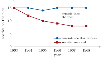
In 1963, on a rocky shore of the Pacific, a young ecologist began throwing every starfish he found on a stretch of rock back into the sea, and kept doing it for years. The starfish ate mussels. Without them, the mussels spread downward over the rock and crowded out the barnacles, limpets, chitons and algae that had lived there; a community of fifteen species fell to eight. One predator, itself neither abundant nor large, had been holding the whole assembly in place. Species do not merely share a place; they compete for it, eat one another, live inside and upon one another, and depend on one another, and the community is the sum of these interactions. This chapter classifies them, gives the quantitative models of competition and predation that a first year can handle, and shows through experiments how one interaction can shape a whole ecosystem.

27.1 A classification of interactions

Definition 27.1 (Interspecific interactions)

An interaction between two species is classified by its effect on each: $+$ (benefit), $-$ (harm) or $0$ . Competition ( $-/-$ ): both use a resource in short supply. Predation ( $+/-$ ): one kills and eats the other; herbivory ( $+/-$ ) when the eaten is a plant and usually survives; parasitism ( $+/-$ ) when the exploiter lives on or in a host it does not kill at once. Mutualism ( $+/+$ ): both benefit. Commensalism ( $+/0$ ): one benefits, the other is unaffected. Amensalism ( $-/0$ ): one is harmed, the other unaffected. Every interaction is a selective pressure on both partners, and their reciprocal adaptation over generations is coevolution.

Example 27.2 (One tree, all six)

An oak competes with its neighbours for light; its acorns are eaten by jays (predation) and its leaves by caterpillars (herbivory); mistletoe draws its sap (parasitism); its roots exchange sugars for phosphate with a fungus (mutualism); ferns grow on its bark, using it only as a perch (commensalism); and its shade kills the grass beneath it (amensalism).

27.2 Competition

Definition 27.3 (Interspecific competition)

Two species compete when they both use a resource — food, light, water, space, nesting sites — whose supply limits their growth. Competition may be by exploitation (each takes what the other would have used) or by interference (direct aggression, toxins, territories). Its outcome follows the competitive exclusion principle: two species that need the same limiting resource in the same way cannot coexist indefinitely in a stable environment; the better competitor eliminates the other. Coexisting competitors therefore differ in niche (niche partitioning) — and where two species overlap they often diverge in form more than where each lives alone (character displacement).

Proposition 27.4 (The Lotka–Volterra competition model)

Let two species grow logistically (Chapter 25) and let each individual of species 2 count as $\alpha$ individuals of species 1 in the use of species 1’s resource, and each of species 1 as $\beta$ of species 2:

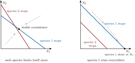
\frac{\dd N_1}{\dd t} = r_1 N_1\left(1 - \frac{N_1 + \alpha N_2}{K_1}\right), \qquad \frac{\dd N_2}{\dd t} = r_2 N_2\left(1 - \frac{N_2 + \beta N_1}{K_2}\right).

Species 1 stops growing on the line $N_1 + \alpha N_2 = K_1$ (its isocline), species 2 on $N_2 + \beta N_1 = K_2$ . If each species limits itself more than it limits the other ( $\alpha < K_1/K_2$ and $\beta < K_2/K_1$ ) the isoclines cross with both species’ equilibrium stable and they coexist; if one isocline lies entirely above the other, that species always excludes the other; if each limits the other more than itself, the winner depends on the starting numbers.

Partial proof. Species 1 grows below its isocline and declines above it; species 2 likewise. When the isoclines cross with species 1’s above species 2’s on the $N_1$ axis and below it on the $N_2$ axis, a point off the crossing is pushed back toward it from every side: the crossing is a stable equilibrium with both species present. When species 1’s isocline lies entirely outside species 2’s, every point where species 2 could still grow is also a point where species 1 grows and it goes on growing after species 2 has stopped, until it reaches $K_1$ with $N_2 = 0$ . The full analysis is done in the Year 2 volume; the sketch of the isoclines gives every outcome without it. ∎

Two outcomes of two-species competition, read from the isoclines (the lines where each species stops growing). Left: the isoclines cross so that each species is held back more by itself than by the other, and they coexist. Right: species 1’s isocline lies outside species 2’s, and species 1 always wins.

Proposition 27.5 (Competitive exclusion)

Two species competing for one limiting resource in a constant environment cannot both persist: the one whose population can keep growing at the lower resource level drives the resource below what the other needs, and the other declines to extinction.

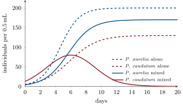
Evidence. Gause (1934) grew two ciliates, Paramecium aurelia and P. caudatum, on a daily ration of bacteria. Alone, each grew logistically to its own plateau. Together, P. aurelia, which grows faster and needs less food per individual, reached nearly its plateau while P. caudatum declined to nothing within sixteen days. A third species, P. bursaria, which feeds at the bottom of the tube where P. aurelia does not, coexisted with it indefinitely: the exclusion held only when the niches were the same. ∎

Gause’s competition experiment (redrawn from his data). Each species alone grows to its plateau; together, P. aurelia rises almost to its own while P. caudatum peaks and is driven to extinction. — Gause’s competition experiment (redrawn from his data). Each species alone grows to its plateau; together, *P. aurelia* rises almost to its own while *P. caudatum* peaks and is driven to extinction.

Example 27.6 (Character displacement in finches)

On islands where a single ground finch lives alone its beak is of middle size; where two species share an island their beaks are respectively smaller and larger than either has alone, each species having shifted toward seeds the other cannot crack. The niches were partitioned by evolution, and the partition is visible in the beak.

27.3 Predation and herbivory

Definition 27.7 (Functional response)

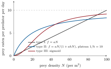
The functional response of a predator is the number of prey one predator eats per unit time as a function of prey density $N$ . Type I: proportional to $N$ (a filter-feeder). Type II: rises then saturates, because each prey takes a handling time $h$ to catch, eat and digest, during which no other can be taken. Type III: sigmoid — low at low density because the predator ignores or cannot find rare prey, then rising steeply (a predator that switches to whatever is common). The numerical response is the change in the number of predators with prey density, through reproduction or immigration.

Theorem 27.8 (The disc equation)

If a predator searches at an attack rate $a$ (area swept per unit time, times the probability of capture) and spends a handling time $h$ on each prey, the number of prey taken per predator per unit time at prey density $N$ is

f(N) = \frac{aN}{1 + ahN} ,

rising linearly as $aN$ at low density and saturating at $1/h$ at high density; $f$ is half its maximum when $N = 1/(ah)$ . In the form $1/f = 1/(aN) + h$ a plot of $1/f$ against $1/N$ is a straight line of slope $1/a$ and intercept $h$ .

Proof. Over a total time $T$ the predator searches for $T_s$ and handles for the rest. Searching, it encounters prey at rate $aN$ , so the number caught is $n = aN T_s$ ; handling them takes $nh$ , so $T = T_s + nh = n/(aN) + nh$ , whence $n/T = aN/(1 + ahN)$ . When $ahN \ll 1$ handling is negligible and $f \approx aN$ ; when $ahN \gg 1$ the predator does nothing but handle and $f \to 1/h$ . Inverting gives the linear form. ∎

Evidence. Holling (1959) had a blindfolded assistant “prey” with a fingertip on sandpaper discs scattered on a table, picking up each found disc (the handling time) before searching again; the number found per minute against disc density gave exactly this curve, and the equation took its name from the experiment. Real predators — a mantis on flies, a stickleback on water fleas — give the same shape, with handling times of seconds to hours. ∎

The three functional responses. Type II saturates at 1/h (here ten prey a day, a handling time of 2.4\, h); type III starts slowly because rare prey are overlooked. — The three functional responses. Type II saturates at $1/h$ (here ten prey a day, a handling time of $2.4\,\mathrm{h}$ ); type III starts slowly because rare prey are overlooked.

Proposition 27.9 (Defences and the arms race)

Prey and plants evolve defences — crypsis, armour, spines, speed, toxins and their warning colours (aposematism), and mimicry: a harmless species copying a toxic one (Batesian) or several toxic species converging on one pattern (Müllerian). Plants defend themselves with thorns, silica, tannins, alkaloids and cyanogenic glycosides, often induced by damage. Predators and herbivores evolve counter-measures — keener senses, detoxifying enzymes, resistance to the toxin — and the pair coevolve. The result is not the destruction of the prey but a running balance: a predator that ate its prey to extinction would follow it.

A predatory sea star on a mussel bed at low tide: the keystone predator whose removal turned a fifteen-species shore into a mussel monoculture.

27.4 Living together: parasitism, mutualism, commensalism

Definition 27.10 (Parasitism, symbiosis, mutualism)

A parasite lives at the expense of a host, on it (ectoparasite: tick, louse, mistletoe) or in it (endoparasite: tapeworm, malaria parasite, rust fungus), taking nutrients and reducing its fitness without necessarily killing it; parasites are often specialised, with complex life cycles through several hosts. A symbiosis is any close, lasting association between two species; a mutualism is one that benefits both: the mycorrhiza (a fungus on or in plant roots, exchanging phosphate and water for sugar; Chapter 23), the root nodule (nitrogen-fixing bacteria fed by the legume), the lichen (a fungus housing an alga or cyanobacterium), the reef coral (a cnidarian housing photosynthetic dinoflagellates), the gut microbiota of a ruminant or a termite (Chapter 22), and pollination (nectar for pollen transport). Many mutualisms began as parasitisms or predations that the partners’ coevolution turned to mutual benefit, and remain conditional: a mycorrhizal fungus in a phosphate-rich soil is a cost, and the plant reduces it.

Example 27.11 (Pollination as a trade)

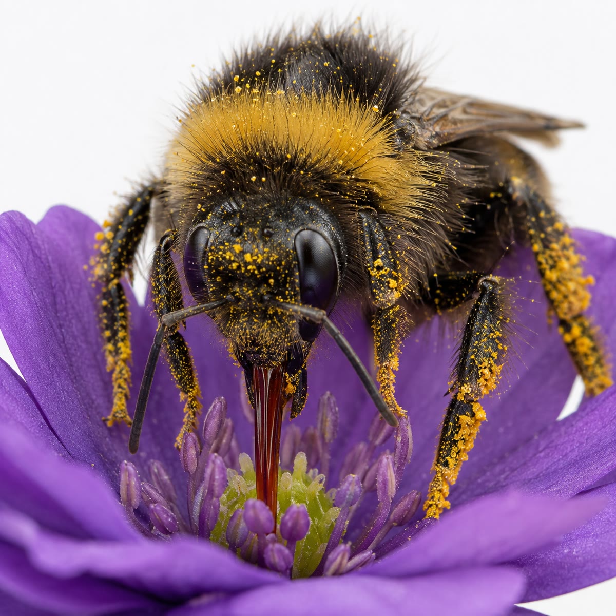
A flower spends a few joules of sugar on nectar; a bee spends flight to collect it and carries pollen between flowers as it goes. The flower’s colour, scent, shape and timing are addressed to its pollinators, and the bee’s tongue length, colour vision and foraging memory to its flowers; some pairs are so tightly fitted — a long nectar spur and the one moth whose tongue reaches it — that neither survives without the other, and a whole plant community can depend on a few species of insect.

A mutualism at work: nectar for the bee, pollen transport for the flower. Each partner’s form has been shaped by the other.

Remark 27.12 (Commensalism is rare and unstable)

Few interactions are truly $+/0$ : the epiphyte that shades its host, the remora that costs its shark a little drag, the cattle egret that eats what the cattle stir up are commensals only to the precision of the measurement. Interactions are classified by their net effect, and the net effect can change with conditions.

27.5 Interactions that shape the community

Definition 27.13 (Keystone species, trophic cascade)

A keystone species is one whose effect on the community is out of proportion to its abundance or biomass: remove it and the community’s structure changes, usually because it controls a dominant competitor. A trophic cascade is the propagation of an effect down a food chain across more than one level: a predator’s presence lowers the herbivores, which raises the plants; its removal does the reverse. Cascades show that communities are structured from the top as well as from the bottom (by productivity, Chapter 26).

Proposition 27.14 (A predator can maintain diversity)

By eating the species that would otherwise win the competition for space or resources, a predator keeps the losers in the community; its removal lets the dominant competitor exclude them, and diversity falls.

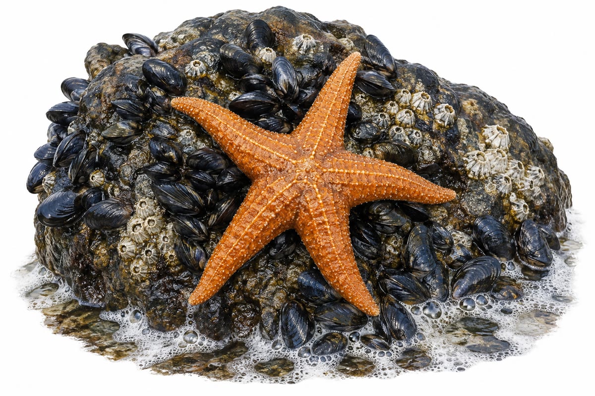
Evidence. Paine (1966) removed the sea star Pisaster from an $8\,\mathrm{m}$ stretch of rocky shore on the Pacific coast of North America and left a neighbouring stretch as control. The sea star eats mussels, barnacles and other sessile animals, mussels by preference. Within two years the mussel Mytilus had spread down the rock and taken nearly all the space; the barnacles, chitons, limpets and algae that had lived in the gaps disappeared, and the fifteen species of the control plot fell to eight. The predator’s own share of the community’s biomass was small; its removal changed everything. ∎

Paine’s removal experiment (after his data). Diversity on the plot without the predator falls by half in five years while the control keeps its fifteen species.

Example 27.15 (Wolves, elk and willows)

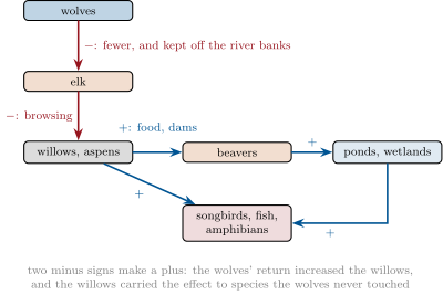
Wolves were exterminated from a large mountain park in the 1920s; its elk multiplied and browsed the willows and aspens along the rivers to stubs; beavers, which need willow, dwindled; songbirds lost their thickets. When wolves were reintroduced in 1995 the elk declined and, more important, avoided the valley bottoms where they were vulnerable; the willows regrew, beavers returned and built dams, and the wetlands they made brought back fish, amphibians and birds. The cascade ran from a carnivore through a herbivore to the plants and from there to a dozen species that never met a wolf — with weather, hunting and other predators contributing, so that the wolves’ share of the change is still debated.

A trophic cascade: an effect passing down three levels and sideways through the community. Signs give the direction of each link.

Wolves and elk in a river valley in winter. The predator’s effect on the vegetation runs through where the elk dare to graze as much as through how many of them there are.

Method 27.16 (Reading an interaction from an experiment)

Identify the manipulation (removal, addition, exclusion cage, pairing in culture) and the control kept alongside it under the same conditions.
For each species, compare its abundance with and without the partner: the sign of the difference gives the sign of the interaction on that species.
Look for indirect effects: a species that changed without touching the manipulated one is at the end of a chain — find the intermediates.
Check the time scale (a competition can take many generations to resolve; a cascade runs at the rate of the slowest level) and the spatial scale (does the result hold beyond the plot?).
Fit the model where the data allow: logistic curves and isoclines for competition, the disc equation for a functional response, and read the parameters off the linearised plots.

27.6 Exercises

Exercise 27.1 ★

Give the sign pair and an example for each of the six kinds of interaction.

Solution

Solution of Exercise 27.1.

Competition $-/-$ (two oaks for light); predation $+/-$ (lynx, hare); parasitism $+/-$ (tick, deer); mutualism $+/+$ (bee, flower); commensalism $+/0$ (fern on bark); amensalism $-/0$ (grass under an oak’s shade).

Exercise 27.2 ★

State the competitive exclusion principle and say why it does not forbid five warblers in one spruce.

Solution

Solution of Exercise 27.2.

Two species using the same limiting resource in the same way cannot coexist indefinitely in a stable environment. The five warblers use the same food but in different parts of the tree and at different times: their niches differ, so no two of them are the “same way”.

Exercise 27.3 ★

Define handling time and attack rate, and give the maximum feeding rate of a predator with $h = 30\,\mathrm{min}$ .

Solution

Solution of Exercise 27.3.

Handling time: the time to catch, eat and digest one prey, during which no other is taken. Attack rate: the area searched per unit time times the probability of capture. Maximum rate $1/h = 2$ prey per hour.

Exercise 27.4 ★

What is a keystone species? Why is a keystone species not simply the most abundant one?

Solution

Solution of Exercise 27.4.

A species whose removal changes the community’s structure out of proportion to its abundance, usually by controlling a dominant competitor. Abundance measures presence, not effect; a rare predator that eats the would-be winner has an effect its numbers do not show.

Exercise 27.5 ★★

Species 1 has $K_1 = 500$ , species 2 has $K_2 = 400$ , with $\alpha = 0.5$ and $\beta = 0.6$ . Draw the isoclines and give the outcome. Repeat with $\alpha = 2$ , $\beta = 0.6$ .

Solution

Solution of Exercise 27.5.

Isocline 1: $N_1 + 0.5 N_2 = 500$ (intercepts 500 on $N_1$ , 1000 on $N_2$ ); isocline 2: $N_2 + 0.6 N_1 = 400$ (400 on $N_2$ , 667 on $N_1$ ). They cross with each species limited more by itself ( $\alpha = 0.5 < K_1/K_2 = 1.25$ ; $\beta = 0.6 < K_2/K_1 = 0.8$ ): stable coexistence at $N_1 = 429$ , $N_2 = 143$ . With $\alpha = 2$ : isocline 1 intercepts 500 and 250, both inside isocline 2’s (667 and 400): species 2 always wins.

Exercise 27.6 ★★

A predator with $a = 0.2\,\mathrm{m}^{2}/\mathrm{h}$ and $h = 0.25\,\mathrm{h}$ meets prey at $10\,$ and $100\,$ per square metre. Compute its feeding rate in each case and the density at which it is half saturated.

Solution

Solution of Exercise 27.6.

$f = aN/(1 + ahN)$ : at 10, $2/(1 + 0.5) = 1.33$ per hour; at 100, $20/(1 + 5) = 3.33$ per hour (maximum $1/h = 4$ ). Half saturation at $N = 1/(ah) = 20$ per square metre.

Exercise 27.7 ★★

Why does a type III response stabilise a prey population at low density while a type II does not?

Solution

Solution of Exercise 27.7.

With a type III response the fraction of prey eaten rises with density at low density: rare prey are taken proportionally less and can recover. With a type II the fraction eaten is highest at low density (the predator is never saturated there), so a small prey population is pushed further down.

Exercise 27.8 ★★

From Gause’s experiment, explain why P. bursaria coexisted with P. aurelia but P. caudatum did not. What made the difference: growth rate or niche?

Solution

Solution of Exercise 27.8.

P. caudatum used the same bacteria in the same water column as P. aurelia, and the faster, more frugal P. aurelia drove the food below what it needed. P. bursaria fed at the bottom on different resources: the niche, not the growth rate, decided — P. bursaria grows no faster than P. caudatum.

Exercise 27.9 ★★

A Batesian mimic becomes more common than its toxic model. Predict what happens to the protection of both, and why the mimic’s success is self-limiting.

Solution

Solution of Exercise 27.9.

Predators meet the pattern more often without harm, learn it less well, and attack it more: protection falls for both mimic and model. The mimic’s fitness therefore falls as it becomes common, a negative frequency dependence that keeps it rare relative to the model.

Exercise 27.10 ★★★

Paine’s removal plot lost seven species. Explain, using the isocline model, how a predator that eats the dominant competitor converts an exclusion into a coexistence.

Solution

Solution of Exercise 27.10.

Without the predator the mussel’s isocline lies outside every competitor’s: it wins the rock. Predation lowers the mussel’s effective $K$ (its isocline is pulled inward) until it crosses the others’ isoclines from the inside: the competitors are now limited more by themselves than by the mussel, and coexist with it. The predator acts on the strongest competitor and makes room for the rest.

Exercise 27.11 ★★★

A mycorrhizal fungus takes $15\,\%$ of a plant’s photosynthate and supplies $80\,\%$ of its phosphate. In what conditions is the association a mutualism, and in what conditions a parasitism? Propose an experiment to tell.

Solution

Solution of Exercise 27.11.

When phosphate limits growth, $80\,\%$ of the phosphate is worth far more than $15\,\%$ of the sugar: mutualism. In a phosphate-rich soil the plant would take up the phosphate itself and the fungus costs $15\,\%$ for nothing: parasitism. Experiment: grow plants with and without the fungus at a range of phosphate levels and measure biomass; the association is mutualistic where the mycorrhizal plants grow larger, parasitic where they grow smaller.

Exercise 27.12 ★★★

Design an experiment to test whether the wolves, rather than the weather or hunting, caused the willows’ recovery: controls, replicates, the variables to measure, and what result would refute the cascade.

Solution

Solution of Exercise 27.12.

Exclosures: fenced plots along the rivers that elk cannot enter, paired with open plots, replicated in several valleys with and without wolf packs, measured for years before and after reintroduction; record willow height and cover, elk density and time spent in each plot (tracks, cameras), hunting and snow depth. The cascade predicts willows recovering in open plots only where wolves are, at the same rate as inside the exclosures; if willows recover equally with and without wolves, or track snow and hunting instead, the cascade is refuted or shared with those factors.

27.7 Problem: The Predator and the Shore

Problem 27.1

Weekend problem — Gause’s ciliates in a tube, a predator’s feeding data fitted to the disc equation, Paine’s shore with and without its sea star, and a pollinator’s budget, ending on the attack rate and handling time of the predator

Part I — Competition in a tube. Two ciliates are grown alone: species A reaches $K_A = 200$ per $0.5\,\mathrm{mL}$ with $r_A = 0.8\,\mathrm{d}^{-1}$ ; species B reaches $K_B = 130$ with $r_B = 0.55\,\mathrm{d}^{-1}$ . Together, an individual of B uses as much food as $\alpha = 1.4$ of A, and an individual of A as much as $\beta = 0.9$ of B.

Write the two isoclines and their intercepts on the axes.
Draw them and state which species wins, and why the outcome does not depend on the starting numbers.
From the doubling times ( $\ln 2/r$ ), which species would you have expected to win from growth rate alone?
A third species C feeds on the bottom of the tube and competes with A only weakly ( $\alpha = 0.3$ , $\beta = 0.3$ , $K_C = 100$ ). Draw the isoclines and give the outcome.
Why does the exclusion principle hold in a tube and so often fail in a forest? Give two reasons.
Compute the equilibrium numbers of A and C from the crossing of the isoclines.

Part II — The disc equation. A predatory beetle is offered prey at densities of 5, 10, 20, 40 and 80 per square metre; it eats 2.0, 3.3, 5.0, 6.7 and 8.0 prey per day respectively.

Plot the feeding rate against density and identify the type of response.
Compute $1/f$ and $1/N$ for each point and plot them.
From the slope and intercept, obtain $a$ and $h$ .
Compute the maximum feeding rate and the half-saturation density.
At which of the five densities does the beetle spend more than half its time handling?
The beetle’s prey grow logistically with $r = 0.1\,\mathrm{d}^{-1}$ and $K = 200$ . At what density is the prey’s growth (per beetle-free square metre) equal to the beetle’s consumption if there is one beetle per square metre? Is this equilibrium stable against a small rise in prey?
A second prey species appears that the beetle handles twice as fast. Predict the change in the beetle’s total intake at high density.

Part III — The shore. On Paine’s control plot the community had 15 species; on the removal plot the count fell 15, 12, 10, 9, 8, 8 over five years, and the mussels’ cover of the rock rose from $20\,\%$ to $85\,\%$ .

Compute the Shannon index of a plot with 15 species at equal abundance, and of one with 8 species where mussels are $85\,\%$ of individuals and the other seven share the rest equally.
By what factor did the diversity fall?
Explain, with the signs of the interactions, why removing a $+/-$ interaction (predation on mussels) strengthened a $-/-$ one (competition for rock).
The sea star was less than $1\,\%$ of the plot’s biomass. Why is biomass a poor guide to a species’ importance?
Predict what would have happened had the sea star’s preferred prey been the rarest species rather than the dominant one.
Propose a way to confirm that it was predation on mussels and not some other effect of the sea star (a caging experiment).

Part IV — A mutualism’s budget. A bee visits 1000 flowers in a day and collects $40\,\mathrm{mg}$ of sugar; each flower gives $40\,\text{µ}\mathrm{g}$ of sugar in nectar and receives pollen from, on average, 3 previous flowers per visit. The plant spends $1\,\%$ of its daily photosynthate ( $4\,\mathrm{mg}$ of sugar per flower) on nectar; a bee’s flight costs $0.5\,\mathrm{mg}$ of sugar per hour of foraging ( $8\,\mathrm{h}$ ).

Compute the bee’s net daily gain of sugar and its energy equivalent at $16\,\mathrm{kJ}/\mathrm{g}$ .
Compute the plant’s daily cost per flower as a fraction of its photosynthate and say what it buys.
Why is this interaction $+/+$ even though each partner is exploiting the other?
A nectar robber bites the base of the flower and takes the nectar without touching the pollen. Give the signs of the robber–plant interaction and its likely effect on the bee.
Draw the sign diagram of plant, bee, robber and a bird that eats robbers, and predict the bird’s indirect effect on the plant.
State the result: the attack rate and handling time of the beetle, and its maximum feeding rate.

Solution

Solution of Problem 27.1.

1. A: $N_A + 1.4 N_B = 200$ , intercepts 200 ( $N_A$ ) and 143 ( $N_B$ ). B: $N_B + 0.9 N_A = 130$ , intercepts 130 ( $N_B$ ) and 144 ( $N_A$ ). 2. The intercepts (200 against 144 on the $N_A$ axis, 143 against 130 on the $N_B$ axis) put A’s isocline entirely outside B’s: solving $N_A = 200 - 1.4 N_B$ with $N_B = 130 - 0.9 N_A$ gives $N_A = -69$ , so the lines meet outside the positive quadrant. A wins from any starting point: wherever B can still grow, A grows too and outlasts it. 3. $T_A = 0.87$ days, $T_B = 1.26$ days: A, the faster grower. 4. A: $N_A + 0.3 N_C = 200$ (200, 667); C: $N_C + 0.3 N_A = 100$ (100, 333). Each species limits itself more than the other ( $0.3 < 200/100$ and $0.3 < 100/200 = 0.5$ ): stable coexistence. 5. A forest is not constant (seasons, disturbances reset the race before it is decided) and has many resources and places, so that species partition niches instead of sharing one. 6. $N_A = 200 - 0.3 N_C$ , $N_C = 100 - 0.3 N_A = 100 - 60 + 0.09 N_C$ , so $N_C = 44$ and $N_A = 187$ . 7. Rising and flattening toward about 10: type II. 8. $(1/N, 1/f)$ : $(0.2, 0.5)$ , $(0.1, 0.303)$ , $(0.05, 0.2)$ , $(0.025, 0.149)$ , $(0.0125, 0.125)$ : a straight line. 9. Slope $(0.5 - 0.125)/(0.2 - 0.0125) = 2.0 = 1/a$ , so $a = 0.5\,\mathrm{m}^{2}/\mathrm{d}$ ; intercept $0.5 - 2\times 0.2 = 0.1$ day $= h$ . 10. Maximum $1/h = 10$ prey per day; half-saturation $N = 1/(ah) = 20$ per square metre. 11. Handling fraction $= f h = f/10$ : more than half when $f > 5$ , i.e. at 40 and 80 per square metre (5.0 at 20 is exactly half). 12. Prey growth $0.1 N (1 - N/200)$ equals consumption $0.5N/(1 + 0.05N)$ : $0.1(1 - N/200) = 0.5/(1 + 0.05 N)$ , i.e. $(1 - N/200)(1 + 0.05N) = 5$ : $1 + 0.05N - N/200 - N^2/4000 = 5$ , so $N^2 - 180 N + 16\,000 = 0$ , $N = 90 \pm \sqrt{8100 - 16\,000}$ : no real root — one beetle per square metre eats more than the prey can ever produce (maximum growth $rK/4 = 5$ per day, at $N = 100$ , where the beetle eats 8.3) and drives it to extinction. No equilibrium; the prey persists only if the beetles are fewer or the prey has refuges. 13. Handling time halves for the second prey ( $h' = 0.05$ ), so at saturation the beetle eats up to 20 of them a day: total intake at high density roughly doubles if it switches to the quicker prey. 14. $H_{15} = \ln 15 = 2.71$ . Eight species: $-(0.85\ln 0.85 + 7\times 0.0214\ln 0.0214) = 0.138 + 0.576 = 0.71$ . 15. By a factor $2.71/0.71 = 3.8$ . 16. The sea star’s $-$ on the mussel kept the mussel’s $-$ on its competitors weak; remove the first and the mussel reaches the density at which its competition excludes the rest. 17. Biomass measures how much of the energy flow a species holds, not what its interactions do; a keystone’s effect goes through the species it controls, whose biomass is large. 18. Removing the sea star would have released a rare species that could not take over the rock: the mussel-dominated community would have been little changed, and the sea star would not have been a keystone. 19. Cages excluding the sea star from small patches, with open cages as controls for the cage’s own effect: if mussels take over only in the closed cages, predation on mussels is the mechanism; cages with the sea star present but mussels removed by hand would test whether the sea star’s other prey matter. 20. Gain $40\,\mathrm{mg}$ , cost $8\times 0.5 = 4\,\mathrm{mg}$ : net $36\,\mathrm{mg}$ $=$ $0.58\,\mathrm{kJ}$ . 21. $40\,\text{µ}\mathrm{g}$ of $4\,\mathrm{mg}$ : $1\,\%$ of the flower’s daily photosynthate buys about three pollen transfers, the plant’s reproduction. 22. Each takes something from the other, but each gains more than it loses: the sign is that of the net effect, not of the exploitation. 23. Robber $+$ , plant $-$ (nectar taken, no pollination): a parasitism of the mutualism; the bee finds emptied flowers and gains less, an indirect $-$ . 24. Plant $\leftrightarrow$ bee $+/+$ ; robber $\to$ plant $-$ , robber $\to$ bee $-$ ; bird $\to$ robber $-$ . Two minus signs: the bird has an indirect $+$ on the plant and on the bee. 25. $a = 0.5\,\mathrm{m}^{2}/\mathrm{d}$ , $h = 0.1\,\mathrm{d}$ ( $2.4\,\mathrm{h}$ ), maximum $10$ prey per day.

Terms defined in this chapter

See all 479 terms in the glossary