University Biology — Year 1 · Bachelor Year 1

28Ecosystem Dynamics

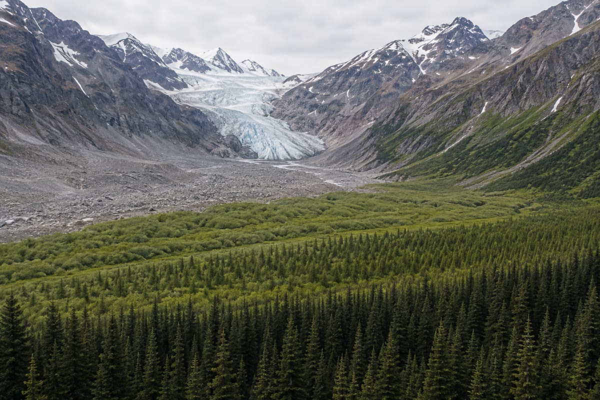
Where a glacier in the north Pacific has been retreating for two centuries, a walk from its snout back down the fjord is a walk through time. The rock uncovered last year is bare; a kilometre on, it wears mosses and a nitrogen-fixing mat; further, thickets of alder; then spruce, then a forest of spruce and hemlock two hundred years old with a metre of soil beneath it. Nothing here is static: ecosystems change after every disturbance, along a path that is partly predictable, and their capacity to hold and recycle their nutrients changes with them. This chapter follows those changes — succession, disturbance and recovery, the retention of nutrients, the assembly of communities on islands — and the experiments that turned them from narratives into numbers.

28.1 Succession

Definition 28.1 (Ecological succession)

Succession is the directional change of a community over time after a disturbance, one set of species replacing another until a relatively stable community, the climax, persists. Primary succession starts on new substrate without soil or living organisms: rock left by a glacier, a lava flow, a dune, a new island. Secondary succession starts where a community has been destroyed but the soil and its seed bank remain: an abandoned field, a burnt or felled forest, a flooded meadow. The first arrivals, pioneer species, are dispersers that tolerate bare ground; late arrivals are competitors that tolerate shade and need soil.

Proposition 28.2 (The mechanisms of replacement)

Each stage of a succession can bring the next about in three ways. Facilitation: the earlier species make the site fit for the later ones — building soil, fixing nitrogen, casting shade, holding moisture — and are then displaced by them. Inhibition: the first occupants hold the site against all comers until they die or are damaged, and what replaces them is whatever arrives then. Tolerance: the later species arrive at the start too, grow slowly and simply outlast the pioneers, whose presence neither helps nor hinders them. Most successions show all three at different stages; primary succession is dominated by facilitation, since the first task is to make a soil.

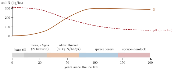
Evidence. At Glacier Bay in Alaska, where the ice has retreated some $100\,\mathrm{km}$ since 1750, the age of each site is known from maps and tree rings, and the stages can be visited in order: bare till, a crust of cyanobacteria and mosses, mats of the nitrogen-fixing Dryas, alder thickets (nitrogen-fixing, adding $50\,\mathrm{kg}$ of nitrogen per hectare per year), then Sitka spruce, then a spruce–hemlock forest after two centuries. Soil nitrogen rises from nearly nothing to $300\,\mathrm{kg}/\mathrm{ha}$ under the alders and the spruces establish only after them; the pH falls from 8 to below 5 as the litter accumulates. Seedlings of spruce planted on the young till grow only if fertilised with nitrogen: the alders are facilitators. ∎

Primary succession at Glacier Bay: the stages in order of site age, with the soil’s nitrogen rising under the nitrogen-fixing alders and the pH falling as litter accumulates. The spruces come in once the alders have built the soil.

A retreating glacier’s valley read as a time series: bare moraine by the ice, then low thickets, then conifer forest on the ground uncovered longest.

Example 28.3 (An old field)

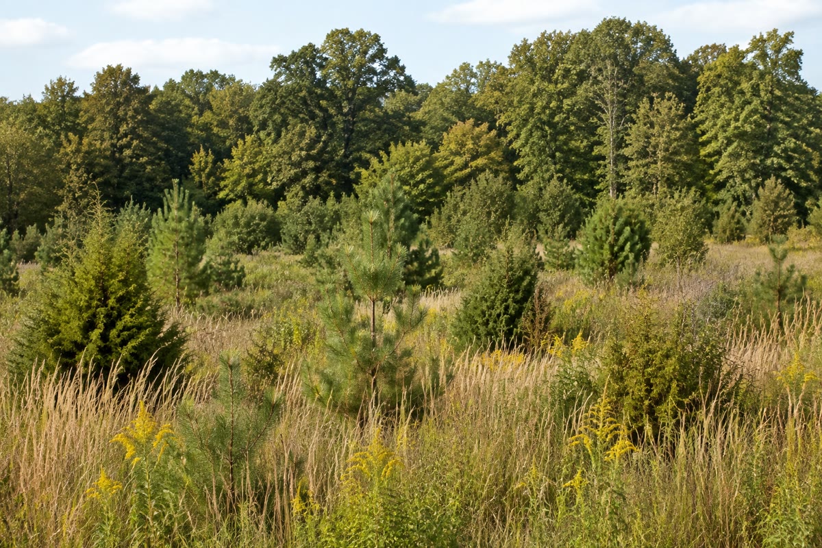
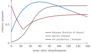
A field abandoned in the eastern United States is colonised the first year by annual weeds (crabgrass, ragweed) from the seed bank and the wind; by the third year perennial herbs and goldenrod dominate; by the tenth, shrubs and pine seedlings; by the twenty-fifth a pine wood, under whose shade the pines’ own seedlings cannot grow but oaks and hickories can; and by the hundredth an oak–hickory forest, whose seedlings tolerate its shade and which therefore replaces itself. Each stage is displaced by species that were worse dispersers and better competitors than itself; the soil was there from the start, and the whole sequence takes a human lifetime rather than the millennia of a primary succession.

Secondary succession in an abandoned field: goldenrod and grasses in front, young pines and junipers behind, and the deciduous forest that will replace them at the back.

Trends through a secondary succession (schematic). Biomass rises to a plateau; species richness peaks mid-way, when pioneers and late species overlap; the ratio of net production to biomass falls as the community fills with wood that costs respiration and adds little growth.

28.2 Disturbance, stability and diversity

Definition 28.4 (Disturbance, resistance, resilience)

A disturbance is an event — fire, storm, flood, drought, grazing, felling, an epidemic — that removes biomass and opens space. An ecosystem’s resistance is its capacity to remain unchanged through a disturbance; its resilience is the speed with which it returns to its former state afterward. A forest is resistant to a dry summer and slow to recover from a fire; a grassland is the reverse. Communities are shaped by their disturbance regime: its frequency, intensity and extent. Many communities are mosaics of patches at different stages of succession since their last disturbance, and their diversity is the sum over the mosaic.

Proposition 28.5 (The intermediate disturbance hypothesis)

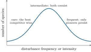
Diversity is highest at intermediate frequencies and intensities of disturbance. Where disturbances are rare the best competitors exclude the rest; where they are frequent only the fastest colonisers survive; between the two, pioneers and competitors coexist, each in the patches that suit it.

Evidence. On rocky shores and coral reefs, the number of species of algae or corals on boulders and reef sections is greatest on those that are overturned or broken by storms at intermediate rates: small boulders (turned often) carry a few pioneer algae, large ones (rarely turned) a monoculture of the best competitor, medium ones the most species. The same hump appears in stream beds against flood frequency and in grasslands against grazing intensity. ∎

The intermediate disturbance hypothesis: diversity peaks where disturbances are frequent enough to prevent competitive exclusion and rare enough to let slow species establish.

Remark 28.6 (Does diversity make an ecosystem stable?)

Grassland plots sown with more species keep their biomass more steadily through droughts than plots with few, because with more species some are always suited to the year’s weather — an insurance effect. But diverse communities are not always more resistant, and the individual populations in them fluctuate as much as anywhere: diversity stabilises the ecosystem’s functions (production, nutrient retention) more than its composition.

28.3 Decomposition and the retention of nutrients

Definition 28.7 (Decomposition and nutrient budget)

Decomposition is the breakdown of dead organic matter (litter, dead wood, corpses, dung) by detritivores and decomposers into carbon dioxide, water and mineral ions — mineralisation. Its rate depends on temperature, moisture, oxygen and the litter’s quality (nitrogen content, lignin): a leaf disappears in a year in a warm wet forest, in a decade under conifers on a cold slope, in millennia in a bog. The mineral ions released are taken up again by roots and microbes, and in a mature ecosystem this internal cycle carries most of the nutrient flow: the input from weathering and rain and the output in stream water are small beside it. A nutrient budget compares inputs, outputs and the internal pools of one element for a defined ecosystem; the biogeochemical cycles at the scale of the planet are treated in the Year 2 volume.

Proposition 28.8 (The living community retains nutrients)

Nutrients are kept in an ecosystem by the uptake of living plants and microbes; when the vegetation is removed, mineralisation continues while uptake stops, and the released ions are washed out into the streams — the ecosystem leaks until a new cover regrows.

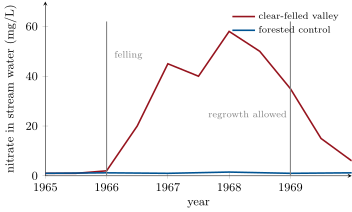
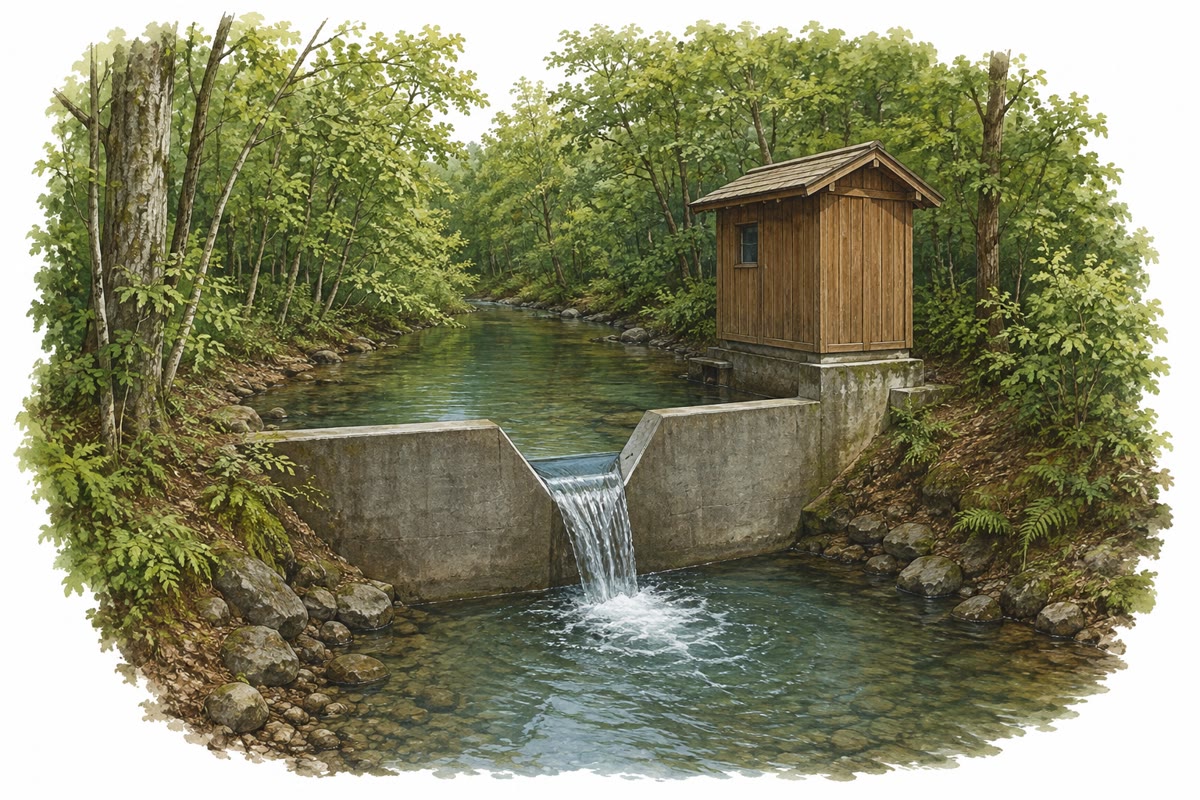
Evidence. At Hubbard Brook in New Hampshire, six small forested valleys are each drained by one stream fitted with a weir, so that everything leaving in the water can be measured against what arrives in the rain. In 1965–66 one valley was clear-felled and kept bare with herbicide for three years, its neighbour left as a control. Stream flow from the cut valley rose by $40\,\%$ (no transpiration). Nitrate in its stream rose forty- to sixtyfold, calcium tenfold, potassium twentyfold; the total loss of dissolved substances was six to eight times the control’s — nitrogen that the intact forest had been holding in its cycle for centuries left in two summers. When regrowth was allowed, the losses fell back within a few years, as fast as the new vegetation took up what the soil released. ∎

The Hubbard Brook clear-felling (after the published stream records, simplified). Nitrate in the stream of the felled valley rose fortyfold while the forested control stayed at a milligram per litre, and fell again once the vegetation regrew.

A gauging weir at the outlet of a forested valley: the only exit for water and dissolved nutrients, where a whole ecosystem’s budget can be measured.

Definition 28.9 (Ecosystem engineers)

An ecosystem engineer is a species that changes the physical environment for others: beavers flood valleys, earthworms mix and aerate the soil, corals and mussels build reefs, trees cast shade and hold water, elephants open forest into grassland, burrowers oxygenate sediments. Engineers act on the biotope rather than through trophic links, and their effect can outlast them (a beaver meadow, a reef, a peat bog).

28.4 Islands and the assembly of communities

Theorem 28.10 (The equilibrium theory of island biogeography)

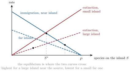
The number of species on an island is a dynamic equilibrium between immigration from a source pool of $P$ species and extinction on the island. If the immigration rate of new species falls linearly with the number $S$ already present, $I = I_0(1 - S/P)$ , and the extinction rate rises linearly with it, $E = eS$ , the equilibrium is

S^* = \frac{I_0 P}{I_0 + eP} ,

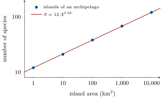
reached when $I = E$ , with a continual turnover of $eS^*$ species per unit time. Islands near the source have a higher $I_0$ and more species; large islands have a lower $e$ (larger populations) and more species. Across a set of islands the number of species rises with area as $S = cA^z$ , a straight line of slope $z$ on a log–log plot, with $z$ typically between $0.2$ and $0.35$ .

Partial proof. $S$ rises while immigration exceeds extinction and falls when extinction exceeds immigration, so $\dd S/\dd t = I_0(1 - S/P) - eS$ is a first-order linear equation whose single equilibrium, $I_0 - (I_0/P + e)S = 0$ , gives $S^*$ and is stable, since the rate of change is positive below it and negative above. At equilibrium species are still arriving and vanishing at the rate $eS^*$ : the number is steady, the list is not. The power law is empirical; its exponent near $0.25$ means that a tenfold larger island holds about $1.8$ times as many species, and that losing $90\,\%$ of a habitat will eventually lose about half its species. ∎

Evidence. Simberloff and Wilson (1969) counted the arthropod species on small mangrove islets off Florida, fumigated the islets to kill every animal, and counted again at intervals. Within a year each islet had recovered close to its original number of species — more on the near and large islets, fewer on the far and small — but with a different list, and the list kept changing: the number was in equilibrium, the composition in turnover, as the theory required. Krakatau, sterilised by its eruption in 1883, had $30$ species of plants after three years and over $270$ after fifty, approaching the richness of similar islands nearby. ∎

The equilibrium model of island biogeography: immigration of new species falls and extinction rises with the number already present. Nearness raises the immigration line, size lowers the extinction line, and each pair of lines fixes an equilibrium.

A species–area relationship on logarithmic axes: a straight line of slope z = 0.25, so that ten times the area holds 1.8 times the species. — A species–area relationship on logarithmic axes: a straight line of slope $z = 0.25$ , so that ten times the area holds $1.8$ times the species.

Proposition 28.11 (Fragmentation)

A habitat cut into fragments behaves like an archipelago: each fragment loses species toward the equilibrium its area and isolation allow, slowly at first (the extinction debt), the large-bodied, rare and specialised species first. Fragments also gain edge — drier, windier, more disturbed — at the expense of interior; a square fragment of $1\,\mathrm{km}^{2}$ with a $100\,\mathrm{m}$ edge zone keeps $64\,\%$ of its area as interior, one of $0.1\,\mathrm{km}^{2}$ only $15\,\%$ . Corridors between fragments raise the immigration rate, which is why they restore species faster than they add area.

Method 28.12 (Using a species–area relationship)

Plot $\log S$ against $\log A$ for a set of islands or fragments sampled with equal effort; fit a line by eye or least squares.
Read $z$ as the slope and $c$ as the value of $S$ at $A = 1$ .
Predict the species of a new area as $cA^z$ ; predict the fraction of species retained when an area is reduced from $A_0$ to $A$ as $(A/A_0)^z$ — with $z = 0.25$ , keeping a tenth of the habitat keeps $56\,\%$ of the species eventually.
Beware: the loss is reached only after the extinction debt is paid, sometimes decades later; and the fit says nothing about which species go.

28.5 Exercises

Exercise 28.1 ★

Distinguish primary from secondary succession with one example of each, and say which is faster and why.

Solution

Solution of Exercise 28.1.

Primary: on new substrate without soil (a moraine, a lava flow); secondary: where soil and seed bank remain (an abandoned field, a burnt wood). Secondary is faster, by a factor of ten or more, because the soil and its nutrients and seeds do not have to be made.

Exercise 28.2 ★

Name the three mechanisms of species replacement and give the one that dominates on a fresh lava flow.

Solution

Solution of Exercise 28.2.

Facilitation, inhibition, tolerance. On lava, facilitation: the pioneers (lichens, mosses, nitrogen fixers) must build soil before anything else can root.

Exercise 28.3 ★

Define resistance and resilience, and classify a coral reef (slow to regrow, easily bleached) and a meadow.

Solution

Solution of Exercise 28.3.

Resistance: remaining unchanged through a disturbance; resilience: returning quickly afterward. A reef is neither resistant to warming nor resilient; a meadow has low resistance to a fire and high resilience.

Exercise 28.4 ★

With $S = 12 A^{0.25}$ , compute the species expected on islands of $16\,\mathrm{km}^{2}$ and $625\,\mathrm{km}^{2}$ .

Solution

Solution of Exercise 28.4.

$16^{0.25} = 2$ : $24$ species; $625^{0.25} = 5$ : $60$ species.

Exercise 28.5 ★★

Why do spruces at Glacier Bay grow on the young till only if fertilised with nitrogen, and what does this prove about the alders?

Solution

Solution of Exercise 28.5.

The till has almost no nitrogen; spruces cannot fix it and grow only where it is supplied. The alders, which fix nitrogen and raise the soil’s content to hundreds of kilograms per hectare, are therefore what makes the site fit for spruce: facilitation.

Exercise 28.6 ★★

A source pool holds 200 species; an island receives $I_0 = 8$ new species a year when empty and loses $e = 0.05$ of its species a year. Compute the equilibrium number and the turnover at equilibrium. Repeat for an island twice as far ( $I_0 = 4$ ).

Solution

Solution of Exercise 28.6.

$S^* = I_0 P/(I_0 + eP) = 1600/(8 + 10) = 89$ species; turnover $eS^* = 4.4$ species a year. With $I_0 = 4$ : $800/14 = 57$ species, turnover $2.9$ .

Exercise 28.7 ★★

Explain, in terms of uptake and mineralisation, why the felled valley at Hubbard Brook lost nitrate rather than organic nitrogen, and why the losses stopped when the vegetation regrew.

Solution

Solution of Exercise 28.7.

Decomposers went on mineralising the litter and humus to ammonium, and nitrifiers converted it to nitrate, a soluble anion the soil does not hold; with no roots taking it up, it was washed out. Regrowth restored uptake: the new plants took the nitrate as fast as it formed, and the stream ran clean again.

Exercise 28.8 ★★

A leaf litter loses $50\,\%$ of its mass in the first year. If the decay is first-order, compute the rate constant and the fraction left after three years; compare with a conifer litter losing $15\,\%$ a year.

Solution

Solution of Exercise 28.8.

$k = \ln 2/1 = 0.69\,\mathrm{yr}^{-1}$ ; after three years $e^{-2.08} = 12.5\,\%$ left. Conifer: $k = -\ln 0.85 = 0.16\,\mathrm{yr}^{-1}$ , half-life $4.3$ years, $61\,\%$ left after three years — the litter accumulates.

Exercise 28.9 ★★

Use the intermediate disturbance hypothesis to predict how the diversity of a grassland changes as grazing rises from none to heavy, and explain both ends.

Solution

Solution of Exercise 28.9.

Ungrazed: tall competitive grasses shade out the rest, few species. Moderate grazing: the dominants are cropped, light reaches the ground, small herbs coexist with grasses: maximum diversity. Heavy grazing: only prostrate, unpalatable or fast-growing species survive the trampling and cropping: few species again.

Exercise 28.10 ★★★

A forest of $1000\,\mathrm{km}^{2}$ is reduced to ten fragments of $10\,\mathrm{km}^{2}$ . With $z = 0.25$ , compute the species expected in one fragment and in all ten if they were fully isolated from one another, compare with the original, and explain why the sum is not the answer.

Solution

Solution of Exercise 28.10.

Original: $c\,1000^{0.25} = 5.6c$ ; one fragment $10^{0.25}c = 1.78c$ , $32\,\%$ of the original. Ten isolated fragments hold, if their lists were entirely different, $17.8c$ — more than the original, which is absurd: the fragments share most species, so the sum overcounts. The true total lies between $1.78c$ (identical lists) and about $5.6c$ (the original), less what the isolation and edges remove; the species lost first are those that need more than $10\,\mathrm{km}^{2}$ each.

Exercise 28.11 ★★★

The Simberloff–Wilson islets recovered their species numbers within a year but with different species. Explain why this supports the equilibrium theory better than an exact recovery of the original list would have.

Solution

Solution of Exercise 28.11.

Exact recovery would suggest a fixed community determined by the island’s conditions; recovery of the number with a different list, and a list that keeps changing, is what a balance between random immigration and extinction predicts — the number is a property of area and distance, the identities are chance.

Exercise 28.12 ★★★

“A climax forest is a closed system.” Discuss with reference to the Hubbard Brook budgets: what enters, what leaves, what is recycled, and what the felling showed about where the retention comes from.

Solution

Solution of Exercise 28.12.

Not closed: it takes in rain, dust, nitrogen from the air (by fixation and deposition) and ions from weathering rock, and loses water, dissolved ions and gases through its stream and its air; but the inputs and outputs are small compared with the internal cycle from litter to soil to root to leaf, so that the forest looks closed to the resolution of a year’s budget. The felling showed where the apparent closure came from: the uptake by living vegetation; with it gone, the same soil and the same decomposers made the valley leak its nutrients in a season.

28.6 Problem: The Felled Valley and the Archipelago

Problem 28.1

Weekend problem — the nutrient budget of a clear-felled valley, and the species–area law of an archipelago, ending on the exponent $z$ and the equilibrium species number of an island

Part I — Reading a succession. A chronosequence of sites of known age since a glacier’s retreat gives: at 10 years, mosses and a mat of nitrogen fixers, soil nitrogen $10\,\mathrm{kg}/\mathrm{ha}$ ; at 40 years, alder thicket, $150\,\mathrm{kg}/\mathrm{ha}$ ; at 80 years, spruce forest, $300\,\mathrm{kg}/\mathrm{ha}$ ; at 200 years, spruce–hemlock, $320\,\mathrm{kg}/\mathrm{ha}$ .

Compute the mean rate of nitrogen accumulation in each interval and say when it is fastest.
Which mechanism of replacement does the nitrogen curve point to, and for which transition?
Why does the accumulation nearly stop after 80 years even though the forest is still alive?
The alder fixes $50\,\mathrm{kg}/\mathrm{ha}$ of nitrogen a year. What fraction of it is retained in the soil between years 40 and 80, and where does the rest go?
Propose an experiment that would distinguish facilitation from tolerance for the alder-to-spruce transition.
Why is a chronosequence a substitute for, and not the same as, watching one site for two centuries?

Part II — The felled valley. Two adjacent valleys of $15\,\mathrm{ha}$ each receive $1300\,\mathrm{mm}$ of rain a year with $6.5\,\mathrm{kg}/\mathrm{ha}$ of nitrogen dissolved in it. The forested control valley exports $820\,\mathrm{mm}$ of stream water a year carrying $2\,\mathrm{kg}/\mathrm{ha}$ of nitrate-nitrogen, $9\,\mathrm{kg}/\mathrm{ha}$ of calcium and $2\,\mathrm{kg}/\mathrm{ha}$ of potassium. The felled valley, in the second year after felling, exports $1150\,\mathrm{mm}$ carrying $120\,\mathrm{kg}/\mathrm{ha}$ of nitrate-nitrogen, $90\,\mathrm{kg}/\mathrm{ha}$ of calcium and $36\,\mathrm{kg}/\mathrm{ha}$ of potassium. Its soil and litter hold $3500\,\mathrm{kg}/\mathrm{ha}$ of nitrogen, the felled biomass another $350\,\mathrm{kg}/\mathrm{ha}$ .

By how much did the water yield rise, and why?
Compute the mean nitrate-nitrogen concentration of each stream in milligrams per litre ( $1\,\mathrm{mm}$ of water over $1\,\mathrm{ha}$ is $10\,\mathrm{m}^{3}$ ).
Compute the nitrogen balance (input minus output) of each valley. Which is accumulating nitrogen, and at what rate?
What fraction of the felled valley’s soil nitrogen left in that one year? At that rate, how long would the pool last?
By what factors did the calcium and potassium exports rise? Why potassium more than calcium (think of where each is held in a soil)?
Where did the exported nitrate come from, given that no vegetation was growing to release it? Name the two microbial steps.
After regrowth is allowed, the export falls to $20\,\mathrm{kg}/\mathrm{ha}$ in year 4 and $5\,\mathrm{kg}/\mathrm{ha}$ in year 6. How long until the rain input again exceeds the output, and what has restored the retention?

Part III — The archipelago. Five islands of $1\,\mathrm{km}^{2}\text{, }10\,\mathrm{km}^{2}\text{, }100\,\mathrm{km}^{2}\text{, }1000\,\mathrm{km}^{2}\text{ and }10\,000\,\mathrm{km}^{2}$ carry $12$ , $21$ , $38$ , $68$ and $120$ species of land birds. The mainland pool is $300$ species.

Compute $\log_{10}$ of each area and each species count and plot them.
Obtain $z$ from the two end points and $c$ from the smallest island; check the middle islands.
Predict the species number of an island of $250\,\mathrm{km}^{2}$ .
The $100\,\mathrm{km}^{2}$ island receives $I_0 = 6$ new species a year when empty and loses a fraction $e$ of its species a year. Using $S^* = 38$ , compute $e$ and the turnover at equilibrium.
An island of the same area twice as far away has $I_0 = 3$ . Compute its equilibrium species number with the same $e$ .
A bridge connects the $100\,\mathrm{km}^{2}$ island to the mainland and $I_0$ rises to $30$ . Compute the new equilibrium and explain why it is still far below $300$ .
If $z$ were $0.35$ instead of $0.25$ , would the small islands have more or fewer species relative to the large? Say what a high $z$ means biologically.

Part IV — Fragmentation and recovery.

A reserve of $1000\,\mathrm{km}^{2}$ is planned in a forest of $100\,000\,\mathrm{km}^{2}$ that is otherwise to be cleared. With $z = 0.25$ , what fraction of the forest’s species can the reserve eventually hold?
Would ten reserves of $100\,\mathrm{km}^{2}$ hold more or fewer, if they are isolated? If they are connected by corridors?
The reserve’s edge zone is $300\,\mathrm{m}$ wide. Compute the interior fraction of a square reserve of $1000\,\mathrm{km}^{2}$ and of one of $100\,\mathrm{km}^{2}$ .
Sketch the number of species of a newly isolated fragment against time, and explain the term extinction debt.
State the result: the exponent $z$ of the archipelago and the equilibrium number of species of the $100\,\mathrm{km}^{2}$ island before and after the bridge.

Solution

Solution of Problem 28.1.

1. 10–40 years: $140/30 = 4.7\,\mathrm{kg}/\mathrm{ha}$ a year; 40–80: $150/40 = 3.75$ ; 80–200: $20/120 = 0.17$ . Fastest in the alder stage. 2. Facilitation, for alder to spruce: the nitrogen the alders add is what the spruces need. 3. The forest has reached a steady state: inputs (fixation, deposition) balance losses (leaching, denitrification, wood removed) and the nitrogen cycles internally rather than accumulating. 4. $150\,\mathrm{kg}/\mathrm{ha}$ retained over 40 years against $2000$ fixed: $7.5\,\%$ ; the rest is held in the alders’ own biomass and litter, leached, or denitrified. 5. Plant spruce seedlings on 20-year till with and without alders and with and without nitrogen fertiliser: if spruce grows without alders when fertilised, and not without fertiliser, the alders’ effect is nitrogen (facilitation); if spruce grows equally in all plots and simply slower than alder, tolerance. 6. It assumes every site started alike and followed the same path, which climate, chance arrivals and the glacier’s varying till may have broken; only a permanent plot proves the sequence at one place. 7. By $330\,\mathrm{mm}$ , $40\,\%$ : the trees no longer transpired their share of the rain. 8. Control: $2\,\mathrm{kg}/\mathrm{ha}$ in $8200\,\mathrm{m}^{3}$ : $0.24\,\mathrm{mg}/\mathrm{L}$ . Felled: $120\,\mathrm{kg}$ in $11\,500\,\mathrm{m}^{3}$ : $10.4\,\mathrm{mg}/\mathrm{L}$ , forty times more. 9. Control: $6.5 - 2 = +4.5\,\mathrm{kg}/\mathrm{ha}$ a year, accumulating. Felled: $6.5 - 120 = -113.5\,\mathrm{kg}/\mathrm{ha}$ a year, losing. 10. $120/3850 = 3.1\,\%$ in a year; the pool would last some $30$ years at that rate — but the rate falls as regrowth returns. 11. Calcium tenfold, potassium eighteenfold. Potassium is held mostly in living tissue and easily leached from litter; calcium is also bound on soil clays and in the rock, released more slowly. 12. From the mineralisation of litter, humus and the felled slash: ammonification (organic N to ammonium) by decomposers, then nitrification (ammonium to nitrate) by nitrifying bacteria, faster in the warmer, wetter, uncovered soil. 13. Falling from $120$ to $20$ to $5$ : below the $6.5\,\mathrm{kg}/\mathrm{ha}$ input by about year 6; the uptake of a new cover of pin cherry, raspberry and saplings restores the retention. 14. $\log A$ : 0, 1, 2, 3, 4; $\log S$ : 1.08, 1.32, 1.58, 1.83, 2.08 — a straight line. 15. $z = (2.08 - 1.08)/4 = 0.25$ ; $c = 12$ . Middle islands: $12\times 10^{0.25} = 21.3$ , $12\times 10^{0.5} = 37.9$ , $12\times 10^{0.75} = 67.5$ : all within one species. 16. $12\times 250^{0.25} = 12\times 3.98 = 48$ species. 17. $38 = 6\times 300/(6 + 300e)$ : $6 + 300e = 47.4$ , $e = 0.138\,\mathrm{yr}^{-1}$ ; turnover $0.138\times 38 = 5.2$ species a year. 18. $3\times 300/(3 + 41.4) = 20$ species. 19. $30\times 300/(30 + 41.4) = 126$ species. Extinction on a $100\,\mathrm{km}^{2}$ island is still fast: even with free access, the species that cannot maintain a population on that area keep dying out; area, not access, sets the ceiling. 20. A higher $z$ means species number falls faster with area: small islands relatively poorer. Biologically, populations on small islands go extinct more readily, or the islands are so isolated that few species reach them (isolation raises $z$ ). 21. $(1000/100\,000)^{0.25} = 0.01^{0.25} = 0.32$ : about a third. 22. Isolated, each holds $(100/100\,000)^{0.25} = 0.18$ of the species; if their lists were independent they would together hold more than the one reserve, but they overlap heavily and each loses the species needing more than $100\,\mathrm{km}^{2}$ , so fewer in practice. Connected by corridors they behave as one $1000\,\mathrm{km}^{2}$ reserve for species that use the corridors: about a third again, with the advantage that a local catastrophe does not empty all of them. 23. $1000\,\mathrm{km}^{2}$ is $31.6\,\mathrm{km}$ a side: interior $(31.6 - 0.6)^2 = 961\,\mathrm{km}^{2}$ , $96\,\%$ . $100\,\mathrm{km}^{2}$ is $10\,\mathrm{km}$ a side: $(10 - 0.6)^2 = 88$ , $88\,\%$ . 24. A slow decline from the original number toward the new equilibrium $cA^z$ , over decades: the species that will go extinct are still present at first, in populations too small to persist — the extinction debt is the difference between the present count and the equilibrium, still to be paid. 25. $z = 0.25$ ; the $100\,\mathrm{km}^{2}$ island holds $38$ species at equilibrium and about $126$ once bridged.

Terms defined in this chapter

See all 479 terms in the glossary