31Field and Lab Methods III

A geophysics crew spends a week in the valley of the Varden Hills, the invented region whose geological map the Year 1 volume drew in its chapter on geological maps. The map shows a granite cropping out on the sides of the valley, between the schists, under the sandstone that rests on both. Where the granite goes under the cover, how far it extends and how deep it reaches, no one has seen. The crew carries a gravimeter, two magnetometers, a cable of electrodes and a radar on a small cart. None of these instruments sees a rock: each measures a field at the surface—gravity, the magnetic field, an electric potential, the echo of a radio pulse—that the rocks below disturb. By the end of the week the crew can draw the granite it never saw, say how deep the alluvium of the valley floor is, and report a magnetic body that no map showed.

This chapter follows that week. It treats each method in turn, as a measurement with its corrections and as a forward problem with a few bodies whose fields can be computed exactly; it then sets out how the errors of a survey add up and why one kind of data rarely fixes a model; and it ends with the Varden survey, where the methods are put together.

You already know

The gravity anomaly, the free-air and Bouguer corrections and anomalies and normal gravity are in the Year 1 volume, in its chapter on isostasy and gravity; the survey loop of a relative gravimeter is described in Chapter 3. The main field, its inclination, the dipole formula and the International Geomagnetic Reference Field are in Chapter 4. Resistivity, Ohm’s law, the relative permittivity, electromagnetic waves, magnetisation and magnetic susceptibility are in the physics books, and Gauss’s theorem for gravity with them. Seismic refraction surveys are in Chapter 2; forward and inverse problems and weighted least squares in Chapter 1; porosity in the school books and wireline logs in Chapter 17. The propagation of uncertainties is in the chemistry and mathematics books.

31.1 Gravity surveys

The anomalies that a gravity survey looks for are small. Gravity at the equator is about $978\,000\,\mathrm{m}\mathrm{Gal}$; large structures change it by hundreds of milligals, a salt dome by about ten, an ore body by about one, and the targets of a geotechnical survey by a few hundredths. Geophysicists measure in milligals, or in gravity units of $0.1\,\mathrm{m}\mathrm{Gal}$; a useful survey must resolve differences of one part in a hundred million of $g$.

Definition 31.1 (Relative gravimeter; instrumental drift)

A relative gravimeter is an instrument that measures differences of gravity between stations: a mass on a spring, kept at a null position by a second, adjustable force whose dial reading, multiplied by a calibration constant, gives gravity in milligals up to an unknown constant. Its instrumental drift is the slow change of its reading at a fixed station, caused by the creep of the spring, temperature and shocks; it is measured by reading again, after a few hours, a station already read, the base station.

A field gravimeter covers a range of several tens of thousands of milligals and reads, at its best, to about $0.01\,\mathrm{m}\mathrm{Gal}$; the range must be reset after transport. At that precision the height of each station matters as much as its reading: $3.3\,\mathrm{cm}$ of height error spoil $0.01\,\mathrm{m}\mathrm{Gal}$, so positions are surveyed with satellite receivers or a level to the centimetre. The base station is re-occupied every couple of hours. The solid-Earth tide, which can reach $0.3\,\mathrm{m}\mathrm{Gal}$, changes slowly enough over those hours to be removed with the drift.

Method 31.2 (Reducing a gravity loop)

A loop starts and ends at a base station, read at times $t_0$ and $t_1$.

1. Compute the drift rate $(r_1 - r_0)/(t_1 - t_0)$ from the two base readings; it includes the tide.
2. Subtract from each reading the drift accumulated since $t_0$, $r - (t - t_0)(r_1 - r_0)/(t_1 - t_0)$, and subtract the base reading: this is gravity relative to the base.
3. Correct for the height $\Delta h$ of the station above the base: add the free-air correction $0.3086\,\mathrm{m}\mathrm{Gal}\,\mathrm{m}^{-1} \times\Delta h$ and subtract the Bouguer correction $0.1119\,\mathrm{m}\mathrm{Gal}\,\mathrm{m}^{-1}\times\Delta h$ (density $2670\,\mathrm{kg}\,\mathrm{m}^{-3}$), that is, add $0.1967\,\Delta h$.
4. For a station a distance $\Delta y$ north of the base, subtract the change of normal gravity, $0.811\,\mathrm{m}\mathrm{Gal}\,\mathrm{km}^{-1} \times\sin 2\varphi\times\Delta y$.
5. Add the terrain correction of each station.

The result is the Bouguer anomaly relative to the base. Tying the base to a station of known absolute gravity gives the anomaly itself.

The Bouguer correction treats the ground between the station and the reference level as a flat slab. In real relief this is wrong twice: a hill that rises above the station pulls upward and lowers the reading, and a valley that falls below it is counted in the slab as rock that is not there.

Definition 31.3 (Terrain correction)

The terrain correction of a gravity station is the attraction that the departures of the relief from the Bouguer slab exert on it: the hills above the level of the station, and the valleys below it, counted with the density of the slab. Both lower the measured gravity compared with the slab, so the correction is always added.

It was computed by hand, with a Hammer chart and tables, zone by zone outward from the station; it is now computed from a digital elevation model. Away from steep relief it rarely exceeds $1\,\mathrm{m}\mathrm{Gal}$, but the zones close to the station are hard to get right, and the correction is seldom known to better than $0.2\,\mathrm{m}\mathrm{Gal}$.

31.1.1 Anomalies of simple bodies

The forward problem of gravity is a sum: each element of a body of density contrast $\Delta\rho$ attracts the station by Newton’s law, and a survey measures the vertical component of the sum. A few bodies give it in closed form.

Theorem 31.4 (Sphere and horizontal cylinder)

At a horizontal distance $x$ from the point above its centre, a buried sphere of excess mass $\Delta m$ whose centre is at depth $z$ gives the anomaly

$$\Delta g(x) = \frac{G\,\Delta m\,z}{(x^2 + z^2)^{3/2}} ,$$

and the anomaly falls to half its peak at $x_{1/2} = z\sqrt{2^{2/3} - 1}$, so that $z = 1.305\,x_{1/2}$. A long horizontal cylinder of excess mass $\lambda$ per unit length, its axis at depth $z$, gives across its strike

$$\Delta g(x) = \frac{2G\lambda z}{x^2 + z^2} ,$$

and $z = x_{1/2}$.

A body that is not a sphere still has a half-width, and the rule then gives the depth of an equivalent sphere, not of the body. The rule is a first guess, made before any model is fitted.

Proposition 31.5 (Vertical cylinder on its axis)

A vertical cylinder of radius $a$ and density contrast $\Delta\rho$, whose top and bottom are at depths $z_1 < z_2$ below the station, gives on its axis

$$\Delta g = 2\pi G\Delta\rho\left[(z_2 - z_1) + \sqrt{z_1^2 + a^2} - \sqrt{z_2^2 + a^2}\right] .$$

For $a \to \infty$ it is the Bouguer slab $2\pi G\Delta\rho(z_2 - z_1)$; for a cylinder from the surface to great depth it tends to $2\pi G\Delta\rho\,a$.

Proposition 31.6 (Excess mass from a gravity map)

Whatever the shape of a body that lies entirely below a horizontal plane, its excess mass is

$$\Delta m = \frac{1}{2\pi G}\iint \Delta g\,\mathrm{d}A ,$$

the integral covering the whole plane.

The theorem gives the mass, never the shape; and a map covers only part of the plane, while the anomaly of a deep body decays slowly, so the mass found from a map is too small unless its edges are extended by a model.

31.1.2 The Varden granite

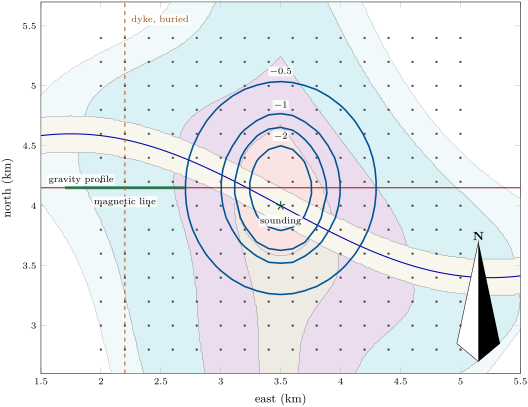
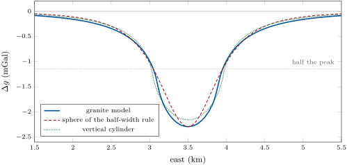
The geologists’ model of the granite is an elliptical body below the unconformity, $760\,\mathrm{m}$ across east–west and $1120\,\mathrm{m}$ north–south where it meets the cover, widening downward; on the valley sides it reaches the surface. Granite is lighter than schist: the published density ranges are $2.50\text{ to }2.81$ and $2.39\text{ to }2.80\,\mathrm{g}\,\mathrm{cm}^{-3}$. The survey’s model takes $2620\,\mathrm{kg}\,\mathrm{m}^{-3}$ for the granite and $2750\,\mathrm{kg}\,\mathrm{m}^{-3}$ for the schist, a contrast of $-130\,\mathrm{kg}\,\mathrm{m}^{-3}$, and stops the granite at $1500\,\mathrm{m}$ below sea level, an assumption since nothing shows its floor. Cut into $5533$ right prisms whose attractions have a closed form, the model gives the anomaly of the map above: a closed low of $-2.29\,\mathrm{m}\mathrm{Gal}$ over the centre of the granite, its contours elongated north–south like the body.

31.2 Magnetic surveys

The Earth’s main field is about $25\,000\,\mathrm{nT}$ at the magnetic equator and about $70\,000\,\mathrm{nT}$ near the magnetic poles. Rocks that hold magnetite add their own field to it, induced by the main field in proportion to their susceptibility, or remanent, carried from the time they formed. A felsic igneous rock has a susceptibility below about $2 \times 10^{-3}$, a mafic one from about $2 \times 10^{-3}$ to $0.4$; on the same scale, one per cent of magnetite by volume gives about $0.03$.

Definition 31.7 (Total-field anomaly; diurnal correction; reduction to the pole)

Let $\mathbf{F}$ be the main field at the survey and $\Delta\mathbf{B}$ the field of the magnetised rocks.

• The total-field anomaly is the measured intensity minus that of the main field, $\Delta T = |\mathbf{F} + \Delta\mathbf{B}| - |\mathbf{F}|$; when $|\Delta\mathbf{B}| \ll |\mathbf{F}|$ it is the projection $\Delta\mathbf{B}\cdot\mathbf{F}/|\mathbf{F}|$.
• The diurnal correction removes the variations of the field with time: a magnetometer at a fixed base station records the field throughout the survey, and each reading $T(t)$ of the moving instrument is replaced by $T(t) - T_\mathrm{base}(t)$.
• The reduction to the pole computes, from the measured anomaly, the anomaly the same rocks would give if the main field were vertical, as at a magnetic pole; the anomaly then sits above its source.

The variations with time come from currents in the ionosphere, about $110\,\mathrm{km}$ up. In a day they typically amount to some $20\text{ to }50\,\mathrm{nT}$, as much as the anomaly of a small target; a magnetic storm can change the field by thousands of nanoteslas. The base station measures the variation, on the assumption that it is the same over the whole survey. The main field itself, or the field of structures larger than the survey, is removed with the IGRF, a constant or a fitted trend.

A proton-precession magnetometer measures the frequency at which proton spins precess in the field, which is proportional to the field; it reads to $1\,\mathrm{nT}$ and needs more than a second per reading. An optically pumped caesium magnetometer is ten to a hundred times more sensitive, reading to $0.01\,\mathrm{nT}$. The stations must be close enough to put at least about three readings across the half-width of the narrowest anomaly sought, and the shallower the source, the closer they must be.

Proposition 31.8 (Anomaly of a thin dyke)

A vertical dyke of thickness $t$ and susceptibility $\kappa$, striking along the magnetic meridian, its top at depth $z$ and extending far down, magnetised by induction in a main field $F$ of inclination $I$, gives across its strike, if $t \ll z$,

$$\Delta T(x) = \frac{\kappa F t\sin^2 I}{2\pi}\,\frac{z}{x^2 + z^2} ,$$

a symmetric anomaly that falls to half its peak at $x = \pm z$: the depth to the top of the dyke is half the full width of the anomaly at half its peak.

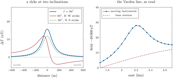
When the dyke strikes across the meridian, the horizontal parts of the magnetisation and of the main field both lie in the plane of the profile, the side faces carry charges, and the anomaly becomes asymmetric, with a low on the side of the pole. The figure below computes it exactly for a dyke of finite width, by adding the closed fields of its four charged faces. The reduction to the pole turns such an anomaly back into the symmetric one of a vertical field.

31.3 Electrical methods

Resistivity ranges more widely than any other property of rocks: unweathered igneous and metamorphic rocks lie between about $1000$ and $100\,000\,\Omega\mathrm{m}$, shales between about $3$ and $30$, dry gravel and sand between a few hundred and ten thousand; fresh water lies between about $1.5$ and $130\,\Omega\mathrm{m}$ and salt water below one. Pore water conducts better than most rock-forming minerals, by its ions, so the current flows mainly through the pores, and the porosity, the saturation and the salinity of the water control the resistivity of a rock.

Theorem 31.9 (Point source on a uniform ground)

A current $I$ injected at a point of the surface of a uniform ground of resistivity $\rho$ produces at a distance $r$ the potential

$$V(r) = \frac{\rho I}{2\pi r} .$$

With two current electrodes A ($+I$) and B ($-I$) and two potential electrodes M and N, the potential difference measured is

$$\Delta V_{MN} = \frac{\rho I}{2\pi}\left(\frac{1}{AM} - \frac{1}{BM} - \frac{1}{AN} + \frac{1}{BN}\right) .$$

Definition 31.10 (Apparent resistivity; electrode array; vertical electrical sounding; electrical resistivity tomography)

• The apparent resistivity of a four-electrode measurement is $\rho_a = K\,\Delta V_{MN}/I$, with the geometric factor $K = 2\pi/(1/AM - 1/BM - 1/AN + 1/BN)$: the resistivity of the uniform ground that would give the same reading.
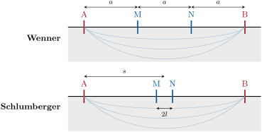
• An electrode array is a rule that places the four electrodes: the Wenner array puts them equally spaced, $a$ apart, in the order AMNB; the Schlumberger array puts M and N, $2l$ apart, at the centre of a much longer AB, of half-length $s$; dipole–dipole, pole–dipole and pole–pole arrays separate the current pair from the potential pair or send one electrode far away.
• A vertical electrical sounding expands an array about a fixed centre and plots $\rho_a$ against the spacing on logarithmic scales: the larger the spacing, the deeper the current flows.
• Electrical resistivity tomography plants many electrodes along a line, measures many four-electrode combinations, and inverts them together for a section of resistivity.

For the Wenner array the factor is $K = 2\pi a$; for the Schlumberger array, $K = \pi(s^2 - l^2)/(2l)$, and $\rho_a \approx 2\pi s^2(-\mathrm{d}V/ \mathrm{d}r)/I$ when $l \ll s$, with $l$ about a tenth of $s$ in practice. A Schlumberger sounding moves only A and B for most readings, the Wenner sounding all four electrodes. The current is a reversing square wave, on, off, reversed, off, for several seconds each, because the ground holds natural self-potentials, of electrochemical origin, that a steady current could not be told from. Small soundings, with electrodes up to about $100\,\mathrm{m}$ apart, need a few hundred milliwatts; soundings a kilometre wide use transmitters of tens of kilowatts.

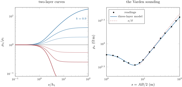
Over layered ground the apparent resistivity of a sounding passes from the resistivity of the top layer, at short spacings, to that of the bottom one, at long spacings. Its curve between the two is the forward problem of the sounding.

Proposition 31.11 (Sounding over layers)

Over horizontal layers of resistivities $\rho_1, \dots, \rho_n$ and thicknesses $h_1, \dots, h_{n-1}$, the Schlumberger apparent resistivity at half-spacing $s$ is

$$\rho_a(s) = s^2\int_0^\infty T(\lambda)\,\lambda\,J_1(\lambda s)\,\mathrm{d}\lambda ,$$

where $J_1$ is the Bessel function of order one and the resistivity transform $T$ is built from the bottom up, $T_n = \rho_n$ and

$$T_i = \frac{T_{i+1} + \rho_i\tanh(\lambda h_i)}{1 + T_{i+1}\tanh(\lambda h_i)/\rho_i} , \qquad T = T_1 .$$

For two layers, with $k = (\rho_2 - \rho_1)/(\rho_2 + \rho_1)$,

$$\frac{\rho_a}{\rho_1} = 1 + 2\sum_{n=1}^{\infty} k^n \left[1 + \left(\frac{2nh_1}{s}\right)^2\right]^{-3/2} ,$$

the sum of the images of the source in the interface and the surface.

The integral form is admitted; the two-layer series follows from Theorem 31.9 by the method of images, the source being reflected again and again, with a factor $k$ each time, in the interface and in the surface.

Proposition 31.12 (A conductive cover on an insulating base)

If layers of total longitudinal conductance $S = \sum_i h_i/\rho_i$ rest on a much more resistive base, the Schlumberger apparent resistivity at spacings much larger than the cover is $\rho_a = s/S$: a straight line of slope one on the logarithmic plot, which gives $S$ but not the thicknesses and resistivities separately.

Proposition 31.13 (Archie’s law)

A clean rock (one free of shale) fully saturated with water of resistivity $\rho_w$ has the resistivity

$$\rho = a\,\rho_w\,\phi^{-m} ,$$

where $\phi$ is its porosity, $a$ a coefficient usually close to $1$ and $m$ the cementation exponent, usually between $1.3$ and $2.8$ when $a = 1$. The ratio $F = \rho/\rho_w$ is the formation factor.

This is Archie’s law, an empirical relation set out by Archie in 1942; it has no proof, only a range of validity. It turns a resistivity into a porosity once the water is known, and the uncertainty of $m$ is the largest in the result.

31.4 Seismic refraction and radar in the field

The seismic refraction survey of Chapter 2 is the field geophysicist’s other way to the depth of a layer: a line of geophones, a weight drop as the source, and the first arrivals plotted against the offset, whose slopes give the velocities and whose intercepts give the depths of the refractors. Over the Varden floor it would see the top of the granite, faster than any sediment above it; it could not see a layer slower than the one above, the blind spot of the method.

Definition 31.14 (Ground-penetrating radar; radargram)

Ground-penetrating radar sends short pulses of radio waves, of frequencies from about $100\,\mathrm{MHz}$ to $1\,\mathrm{GHz}$ and durations of a few nanoseconds, from an antenna on the ground, and records the echoes from contrasts of permittivity and conductivity below. A radargram is the display of the recorded traces side by side along the profile, the two-way travel time increasing downward.

Proposition 31.15 (Radar velocity, reflection and penetration)

In a non-magnetic ground whose conductivity $\sigma$ is small compared with $\omega\varepsilon$, the radar pulse travels at

$$V = \frac{c}{\sqrt{\varepsilon_r}} ,$$

an interface between relative permittivities $\varepsilon_1$ and $\varepsilon_2$ reflects at normal incidence the fraction $R = (\sqrt{\varepsilon_1} - \sqrt{\varepsilon_2})/(\sqrt{\varepsilon_1} + \sqrt{\varepsilon_2})$ of the amplitude, and the amplitude falls by a factor $\mathrm{e}$ over the skin depth

$$\delta = \frac{2}{\sigma}\sqrt{\frac{\varepsilon_0\varepsilon_r}{\mu_0}} \approx 0.0053\,\mathrm{S}\times\frac{\sqrt{\varepsilon_r}}{\sigma} .$$

Velocities run from $0.3\,\mathrm{m}\,\mathrm{ns}^{-1}$ in air to about $0.15$ in dry sand, $0.13$ in granite and $0.06$ in saturated sand or clay, where the permittivity of the water dominates. The useful depth is about three skin depths: in a limestone of permittivity 6 and conductivity $1\,\mathrm{mS}\,\mathrm{m}^{-1}$ the skin depth is about $13\,\mathrm{m}$, in a clay of permittivity 20 and $10\,\mathrm{mS}\,\mathrm{m}^{-1}$ about $2.4\,\mathrm{m}$. A layer is seen if it is at least a quarter of a wavelength thick, so higher frequencies give sharper pictures of shallower ground.

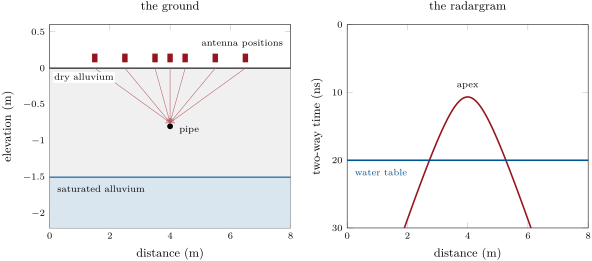
Proposition 31.16 (Diffraction hyperbola)

An antenna moved along the surface above a small buried object at $(x_p, d)$, in ground of velocity $V$, records its echo at the two-way time

$$t(x) = \frac{2}{V}\sqrt{(x - x_p)^2 + d^2} ,$$

a hyperbola with apex $t_0 = 2d/V$ over the object. Any other point $(x, t)$ of it gives $V = 2|x - x_p|/\sqrt{t^2 - t_0^2}$, and then $d = Vt_0/2$.

31.5 Processing and uncertainty

Every number in a survey carries an error, and the reduction adds the errors of the corrections to that of the reading. When the errors are independent, their variances add.

Method 31.17 (An error budget)

1. List the independent sources of error of the reduced value: the reading, the position and height, the density or susceptibility assumed, the drift or diurnal model, the terrain.
2. Convert each into the unit of the result, multiplying by the derivative of the reduction with respect to it.
3. Add the squares and take the square root.
4. Compare the total with the size of the anomaly sought: if it is larger, improve the largest term first.

A model is judged by how well it reproduces the data, and the measure must weigh each datum by its uncertainty.

Definition 31.18 (Data misfit)

The misfit of a model to $N$ data $d_i$ of standard deviations $\sigma_i$ is

$$\chi^2 = \sum_{i=1}^N\left(\frac{d_i - d_i^{\,\mathrm{model}}}{\sigma_i}\right)^2 .$$

A model that explains the data to within their errors has $\chi^2$ close to $N$; a much larger value means the model is wrong, a much smaller one that it fits the noise.

Minimising the misfit is the weighted least squares of Chapter 1. The difficulty of the potential methods is that many models reach the same misfit. Outside a body, its gravity is that of an infinity of others: every sphere with the same excess mass and centre gives the same anomaly, whatever its radius and density; a gravity map fixes the excess mass, but not the shape; a sounding over a conductive cover fixes the conductance $S$, but not the thicknesses; the anomaly of a thin dyke fixes the product $\kappa t$, but not $\kappa$ and $t$ apart. An inversion chooses among the equivalent models by adding information: a density measured on samples, a depth from a borehole, a smoothness imposed on the model. The surest addition is another method, sensitive to another property: gravity sees density, magnetics magnetite, resistivity water, radar permittivity, and each sees what the others miss.

31.6 A mapping project

In the field — A week in the valley

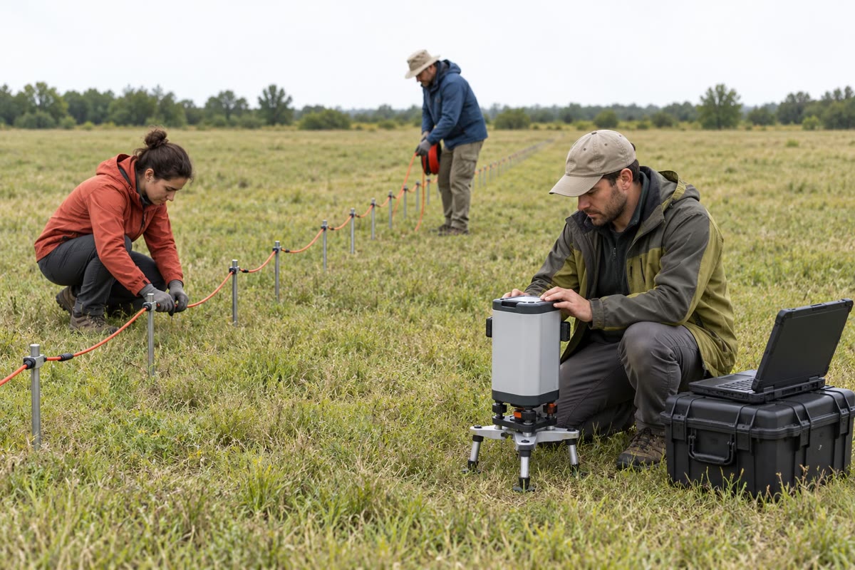
The crew of the Varden survey divides its week among the methods. One member carries the gravimeter round a grid of stations $200\,\mathrm{m}$ apart, levelling it at each, while a colleague surveys the heights with a satellite receiver; every two hours they return to the base station by the bridge. A magnetometer is left at a base station away from the power line and the road, recording all day, while a second is walked along the lines. On the valley floor two others lay out the cable, push the steel electrodes into the alluvium and expand a sounding from a few metres to two hundred; a small radar on a cart is pulled along the floor. In the evening the readings are reduced, and the next day’s lines are chosen from the maps of the day before.

Example 31.19 (The Varden survey)

The gravity map shows a closed low of about $-2.3\,\mathrm{m}\mathrm{Gal}$ centred on the granite, elongated north–south: the light granite continues under the cover, and is longest in that direction. The low extends to about $1\,\mathrm{km}$ from the outcrop, so the body widens with depth. Its half-width gives a first depth for an equivalent sphere; models with a vertical side and a floor show that a floor between one and a few kilometres deep explains the peak equally well, within a few tenths of a milligal, so the floor stays unknown—the non-uniqueness of the previous section. On the valley floor above the granite, the sounding starts at the resistivity of dry gravel, dips where the current enters the water-saturated alluvium and rises along a straight line of slope one: a conductive cover over a highly resistive base, the granite, a few metres down. Radar pulled along the same floor shows a flat echo at about $20\,\mathrm{ns}$: the water table. And the magnetic line across the west limb of the fold, where the cover is thick and the basement schists lie a couple of hundred metres down, records a symmetric high of about $20\,\mathrm{nT}$ that no map explains: a mafic dyke, rich in magnetite, buried under the cover; its strike along the magnetic meridian is why the anomaly is symmetric. The geophysicists report it as a dolerite dyke cut off at the unconformity, which the cover of the map conceals. The weekend problem reduces the data of the survey.

31.7 Exercises

Exercise 31.1 ★

(a) What fraction of $g = 9.81\,\mathrm{m}\,\mathrm{s}^{-2}$ is $0.01\,\mathrm{m}\mathrm{Gal}$? (b) By how much must a gravimeter be raised for its reading to change by $0.01\,\mathrm{m}\mathrm{Gal}$ through the free-air effect alone? (c) Through the free-air and Bouguer effects together, with the density $2670\,\mathrm{kg}\,\mathrm{m}^{-3}$?

Solution

Solution of Exercise 31.1.

(a) $0.01\,\mathrm{m}\mathrm{Gal} = 10^{-7}\,\mathrm{m}\,\mathrm{s}^{-2}$, and $10^{-7}/9.81 = 1.0 \times 10^{-8}$: one part in a hundred million.

(b) $0.01/0.3086 = 0.032\,\mathrm{m}$, about $3.2\,\mathrm{cm}$.

(c) Together the two effects change gravity by $0.1967\,\mathrm{m}\mathrm{Gal}\,\mathrm{m}^{-1}$, the difference $0.3086 - 0.1119$, so the height must change by $0.01/0.1967 = 5.1\,\mathrm{cm}$.

Exercise 31.2 ★

A sphere of radius $50\,\mathrm{m}$ and density contrast $+500\,\mathrm{kg}\,\mathrm{m}^{-3}$ has its centre $100\,\mathrm{m}$ deep. Compute its excess mass, the peak of its anomaly and the half-width $x_{1/2}$.

Solution

Solution of Exercise 31.2.

$\Delta m = \tfrac43\pi(50\,\mathrm{m})^3\times500\,\mathrm{kg}\,\mathrm{m}^{-3} = 2.62 \times 10^{8}\,\mathrm{kg}$. The peak is $G\Delta m/z^2 = 6.674 \times 10^{-11}\times2.62 \times 10^{8}/10^{4} = 1.75 \times 10^{-6}\,\mathrm{m}\,\mathrm{s}^{-2}$, that is $0.175\,\mathrm{m}\mathrm{Gal}$. The half-width is $x_{1/2} = z/1.305 = 77\,\mathrm{m}$.

Exercise 31.3 ★

A Wenner array of spacing $a = 10\,\mathrm{m}$ injects $0.1\,\mathrm{A}$ and measures $0.239\,\mathrm{V}$. (a) Compute the geometric factor and the apparent resistivity. (b) Show that a Schlumberger array with $s = 15\,\mathrm{m}$ and $l = 5\,\mathrm{m}$ has the same geometric factor, and explain why.

Solution

Solution of Exercise 31.3.

(a) With $AM = MN = NB = a$, $K = 2\pi/(1/a - 1/2a - 1/2a + 1/a) = 2\pi a = 62.83\,\mathrm{m}$, and $\rho_a = 62.83\times0.239/0.1 = 150\,\Omega\mathrm{m}$. (b) $K = \pi(15^2 - 5^2)/(2\times5) = \pi\times 200/10 = 62.83\,\mathrm{m}$. The electrodes are then at $0$, $10$, $20$ and $30\,\mathrm{m}$, in the order AMNB: it is the Wenner array of spacing $10\,\mathrm{m}$.

Exercise 31.4 ★

Granite has $\varepsilon_r = 5$. (a) Compute the radar velocity. (b) A fracture lies $10\,\mathrm{m}$ down: compute the two-way time of its echo. (c) With $\sigma = 1\,\mathrm{mS}\,\mathrm{m}^{-1}$, compute the skin depth and the useful depth of about three skin depths. (d) Compare with a wet clay of $\varepsilon_r = 20$ and $\sigma = 10\,\mathrm{mS}\,\mathrm{m}^{-1}$.

Solution

Solution of Exercise 31.4.

(a) $V = 0.2998/\sqrt5 = 0.134\,\mathrm{m}\,\mathrm{ns}^{-1}$. (b) $t = 2\times10/0.134 = 149\,\mathrm{ns}$. (c) $\delta = 0.0053\sqrt5/10^{-3} = 11.9\,\mathrm{m}$, and a useful depth of about $36\,\mathrm{m}$. (d) In the clay $\delta = 0.0053\sqrt{20}/0.01 = 2.4\,\mathrm{m}$, a useful depth of about $7\,\mathrm{m}$, and a velocity of only $0.067\,\mathrm{m}\,\mathrm{ns}^{-1}$. The approximation still holds there: at $100\,\mathrm{MHz}$, $\omega\varepsilon = 2\pi\times10^{8}\times20\times8.85 \times 10^{-12} = 0.11\,\mathrm{S}\,\mathrm{m}^{-1}$, ten times $\sigma$.

Exercise 31.5 ★★

(a) Derive the anomaly of a long horizontal cylinder of radius $R$ and density contrast $\Delta\rho$, its axis at depth $z$, from that of a line mass, and show that $z = x_{1/2}$. (b) A cylinder and a sphere give the same peak and the same half-width $x_{1/2} = 100\,\mathrm{m}$. Compare their depths. Which interpretation gives the deeper body?

Solution

Solution of Exercise 31.5.

(a) The cylinder has $\lambda = \pi R^2\Delta\rho$ per unit length, and outside it its attraction is that of a line mass on its axis (Gauss’s theorem on a coaxial cylinder): $\Delta g = 2G\pi R^2\Delta\rho\,z/(x^2 + z^2)$. Half the peak is reached when $x^2 + z^2 = 2z^2$, so $z = x_{1/2}$. (b) The sphere is at $1.305\times100 = 130\,\mathrm{m}$, the cylinder at $100\,\mathrm{m}$: the same profile, read as a sphere, places the body $30\,\%$ deeper. A sphere’s anomaly decays faster with distance, so a sphere must be deeper to be as wide.

Exercise 31.6 ★★

The Bouguer anomaly of the Varden granite model, sampled every $100\,\mathrm{m}$ on a map of $1120$ points covering $3.5\,\mathrm{km} \times 3.2\,\mathrm{km}$, sums to $-438\,\mathrm{m}\mathrm{Gal}$. (a) Apply Proposition 31.6 to estimate the mass deficit. (b) The model’s mass deficit is $1.74 \times 10^{11}\,\mathrm{kg}$. What fraction does the map recover, and where is the rest?

Solution

Solution of Exercise 31.6.

(a) Each point stands for $100\,\mathrm{m}\times100\,\mathrm{m} = 10^{4}\,\mathrm{m}^{2}$, so $\iint\Delta g\,\mathrm{d}A \approx -438 \times 10^{-5}\times10^{4} = -43.8\,\mathrm{m}^{3}\,\mathrm{s}^{-2}$, and $\Delta m = -43.8/(2\pi\times6.674 \times 10^{-11}) = -1.04 \times 10^{11}\,\mathrm{kg}$. (b) $1.04/1.74 = 60\,\%$. The rest is in the flanks of the anomaly outside the map: the granite reaches a depth of more than a kilometre, and the anomaly of its deep part decays slowly with distance. Extending the map far enough, or a model, recovers it.

Exercise 31.7 ★★

(a) A thin dyke has its top $30\,\mathrm{m}$ down. Using the rule of three readings per half-width, where the half-width is the full width of the anomaly at half its peak, what station spacing does it need? (b) The same for a top $220\,\mathrm{m}$ down. (c) Why can a single survey not resolve both a shallow and a deep body unless it is designed for the shallow one?

Solution

Solution of Exercise 31.7.

(a) For a thin dyke the anomaly falls to half its peak at $x = \pm z$: its full width at half the peak is $2z = 60\,\mathrm{m}$, and three readings across it need a spacing of at most $20\,\mathrm{m}$. (b) $2\times 220/3 = 147\,\mathrm{m}$. (c) The station spacing needed scales with the depth of the shallowest body of interest: a survey designed for the deep dyke, at $150\,\mathrm{m}$, would alias the anomaly of the shallow one, which is only $60\,\mathrm{m}$ wide; one designed for the shallow body sees the deep one too, with many more readings than it needs.

Exercise 31.8 ★★

A sandstone saturated with water of $8\,\Omega\mathrm{m}$ has a resistivity of $80\,\Omega\mathrm{m}$. (a) With $a = 1$ and $m = 2$, compute its porosity. (b) Repeat with $m = 1.8$ and $m = 2.2$. Which term of the measurement controls the uncertainty of the porosity?

Solution

Solution of Exercise 31.8.

(a) $F = 80/8 = 10$ and $\phi = F^{-1/m} = 10^{-1/2} = 0.316$. (b) $10^{-1/1.8} = 0.278$ and $10^{-1/2.2} = 0.351$. A change of $0.2$ in $m$ moves the porosity by about four percentage points; the resistivities, measured to a few per cent, move it much less. The cementation exponent controls the uncertainty, and it must be calibrated on samples of the same rock.

Exercise 31.9 ★★

(a) Compute the first three terms of the two-layer series of Proposition 31.11 at $s = 2h_1$ for $k = 0.5$ and $k = -0.5$, and the apparent resistivities they give. (b) What are the limits of $\rho_a/\rho_1$ for $s \ll h_1$ and $s \gg h_1$? (c) What resistivity ratios $\rho_2/\rho_1$ correspond to $k = \pm 0.5$?

Solution

Solution of Exercise 31.9.

(a) At $s = 2h_1$, $(2nh_1/s)^2 = n^2$, so the terms are $k^n(1 + n^2)^{-3/2}$: $0.3536k$, $0.0894k^2$, $0.0316k^3$. For $k = 0.5$: $0.1768$, $0.0224$, $0.0040$, and $\rho_a/\rho_1 \approx 1 + 2\times0.2031 = 1.406$ (the full sum gives $1.409$). For $k = -0.5$ the terms alternate in sign, $-0.1768 + 0.0224 - 0.0040$, and $\rho_a/\rho_1 \approx 0.683$ (full sum $0.685$). (b) For $s \ll h_1$ every term vanishes and $\rho_a \to \rho_1$; for $s \gg h_1$ every bracket tends to 1 and $1 + 2\sum k^n = 1 + 2k/(1 - k) = (1 + k)/(1 - k) = \rho_2/\rho_1$. (c) $\rho_2/\rho_1 = (1 + k)/(1 - k) = 3$ and $1/3$.

Exercise 31.10 ★★★

(a) Derive the geometric factor of the Wenner array from Theorem 31.9. (b) Derive that of the Schlumberger array, and show that $\rho_a \to 2\pi s^2(-\mathrm{d}V/ \mathrm{d}r)/I$ as $l/s \to 0$. (c) By how much does the approximate factor $\pi s^2/(2l)$ overestimate the exact one when $l = s/10$?

Solution

Solution of Exercise 31.10.

(a) In the order AMNB with spacing $a$: $AM = a$, $BM = 2a$, $AN = 2a$, $BN = a$, so the bracket is $2/a - 1/a = 1/a$ and $K = 2\pi a$. (b) With A and B at $\mp s$ and M and N at $\mp l$: $AM = BN = s - l$, $BM = AN = s + l$, the bracket is $2/(s - l) - 2/(s + l) = 4l/(s^2 - l^2)$, and $K = \pi(s^2 - l^2)/(2l)$. When $l \ll s$, $\Delta V_{MN} \approx 2l\,E$ with $E = 2(-\mathrm{d}V/\mathrm{d}r)$ at the centre, the field of both current electrodes; then $\rho_a = K\Delta V/I \to \pi s^2/(2l)\times 4l(-\mathrm{d}V/\mathrm{d}r)/I = 2\pi s^2(- \mathrm{d}V/\mathrm{d}r)/I$. (c) The ratio of the approximate to the exact factor is $s^2/(s^2 - l^2) = 1/(1 - 0.01) = 1.010$: one per cent.

Exercise 31.11 ★★★

A station stands $50\,\mathrm{m}$ above the base. Its reading is good to $0.01\,\mathrm{m}\mathrm{Gal}$, its height to $5\,\mathrm{cm}$; the density of the slab is uncertain by $100\,\mathrm{kg}\,\mathrm{m}^{-3}$, the terrain correction by $0.2\,\mathrm{m}\mathrm{Gal}$. (a) Draw up the error budget of its Bouguer anomaly. (b) Which term dominates, and which would you improve to detect a $0.1\,\mathrm{m}\mathrm{Gal}$ anomaly? (c) What is the total without the terrain term?

Solution

Solution of Exercise 31.11.

(a) Reading: $0.010\,\mathrm{m}\mathrm{Gal}$. Height: $0.1967\times0.05 = 0.010\,\mathrm{m}\mathrm{Gal}$. Density: the Bouguer correction is $0.04191\,h\,d$ with $d$ in $\mathrm{g}\,\mathrm{cm}^{-3}$, so $0.04191\times50\times0.1 = 0.210\,\mathrm{m}\mathrm{Gal}$. Terrain: $0.200\,\mathrm{m}\mathrm{Gal}$. Total: $\sqrt{0.010^2 + 0.010^2 + 0.210^2 + 0.200^2} = 0.29\,\mathrm{m}\mathrm{Gal}$. (b) The density and the terrain dominate, each about twenty times the reading error. To detect $0.1\,\mathrm{m}\mathrm{Gal}$, the density of the slab must be measured on samples or fitted to the data (the value that least reflects the topography), and the terrain corrected from a fine elevation model. (c) $\sqrt{0.010^2 + 0.010^2 + 0.210^2} = 0.21\,\mathrm{m}\mathrm{Gal}$.

Exercise 31.12 ★★★

Five gravity readings across a buried body, at $x = -600$, $-300$, $0$, $300$ and $600\,\mathrm{m}$, are $-0.69$, $-2.17$, $-4.16$, $-2.10$ and $-0.73\,\mathrm{m}\mathrm{Gal}$, each with $\sigma = 0.03\,\mathrm{m}\mathrm{Gal}$. (a) For sphere models centred under $x = 0$ at depths of $300$, $400$ and $500\,\mathrm{m}$, choose the mass that fits the central reading and compute the misfit $\chi^2$ of each. (b) Which model fits the data within their errors? (c) Could a body of another shape fit as well? What would decide?

Solution

Solution of Exercise 31.12.

(a) The mass that fits the central reading is $\Delta m = \Delta g(0)z^2/G = -4.16 \times 10^{-5}z^2/6.674 \times 10^{-11}$: $-5.61 \times 10^{10}\,\mathrm{kg}$ at $300\,\mathrm{m}$, $-9.97 \times 10^{10}\,\mathrm{kg}$ at $400\,\mathrm{m}$, $-1.56 \times 10^{11}\,\mathrm{kg}$ at $500\,\mathrm{m}$. The predicted readings at $x = \pm300$ and $\pm600$ are $-1.47$ and $-0.37$, $-2.13$ and $-0.71$, $-2.62$ and $-1.09\,\mathrm{m}\mathrm{Gal}$. The misfits are $\chi^2 = 1238$, $3.7$ and $856$. (b) Only the model at $400\,\mathrm{m}$, with $\chi^2 = 3.7$ for five data, fits within the errors. (c) Yes: any spherically symmetric body with the same mass and centre gives exactly the same anomaly, and other shapes can come within the errors. A density measured on samples, a borehole or another method would decide.

31.8 Problem: The hidden bodies of the Varden Hills

Problem 31.1

Weekend problem — reducing the Varden survey

Use $G = 6.674 \times 10^{-11}\,\mathrm{m}^{3}\,\mathrm{kg}^{-1}\,\mathrm{s}^{-2}$, the free-air gradient $0.3086\,\mathrm{m}\mathrm{Gal}\,\mathrm{m}^{-1}$ and the Bouguer factor $0.1119\,\mathrm{m}\mathrm{Gal}\,\mathrm{m}^{-1}$ (density $2670\,\mathrm{kg}\,\mathrm{m}^{-3}$).

Part I — A gravity loop. A loop on the gravity profile gives (readings in milligals after calibration, heights in metres, times in hours after 09:00):

station	base	$3.0\,\mathrm{km}$	$3.5\,\mathrm{km}$	$4.0\,\mathrm{km}$	base
time	0	0.5	0.9	1.3	2.0
height	176.1	149.0	145.5	158.0	176.1
reading	2846.512	2851.075	2850.497	2849.392	2846.708

1. Compute the drift rate of the loop.
2. Correct the three station readings for drift and express them relative to the base.
3. Apply the free-air and Bouguer corrections for the height differences, and give the Bouguer anomaly of each station relative to the base.
4. The drift of the instrument alone was $0.040\,\mathrm{m}\mathrm{Gal}\,\mathrm{h}^{-1}$. What caused the rest of the change at the base, and why could it be removed with the drift?
5. The model the readings come from gives the three anomalies relative to the base as $-0.825$, $-2.131$ and $-0.825\,\mathrm{m}\mathrm{Gal}$. Compute the errors of the reduction. The heights in the table are rounded to $0.1\,\mathrm{m}$: what error can this rounding introduce, and does it explain the errors?
6. What height accuracy keeps the reduced anomaly within $0.01\,\mathrm{m}\mathrm{Gal}$? Why do survey manuals ask for $3.3\,\mathrm{cm}$, a tighter figure?

Part II — The anomaly of the granite. Along the profile the anomaly has its minimum, $-2.293\,\mathrm{m}\mathrm{Gal}$, at $x = 3.50\,\mathrm{km}$, and crosses half that value at $x = 3.048$ and $3.952\,\mathrm{km}$. The granite model has a density contrast of $-130\,\mathrm{kg}\,\mathrm{m}^{-3}$, and the ground at the centre is $145.5\,\mathrm{m}$ above sea level.

7. Compute the half-width $x_{1/2}$ and the depth of the centre of the equivalent sphere.
8. Compute the mass deficit of that sphere, and its radius for the density contrast of the granite. What is odd about the result?
9. The model’s centre of mass is $864\,\mathrm{m}$ below the ground and its mass deficit $1.74 \times 10^{11}\,\mathrm{kg}$. Why does the half-width rule give a shallower and lighter body?
10. A vertical cylinder of the same area as the granite at the unconformity has radius $461\,\mathrm{m}$. Compute its anomaly on the axis for a top at the ground and a floor at $1645\,\mathrm{m}$ depth, and for an unlimited depth.
11. Find, by trial or by solving, the floor depth for which this cylinder gives the observed $-2.29\,\mathrm{m}\mathrm{Gal}$.
12. Compute the cylinder’s anomaly with its top $6\,\mathrm{m}$ down (floor $1645\,\mathrm{m}$). Can gravity tell whether the granite reaches the surface under the alluvium?

Part III — The valley floor. The Schlumberger sounding on the floor above the granite gives (half-spacing $s$ in metres, $\rho_a$ in $\Omega\mathrm{m}$):

$s$	1	2	4	6	10	20	30	40
$\rho_a$	577	526	387	350	449	821	1309	1684

On a radar profile along the same floor, a pipe gives a hyperbola with its apex at $10.7\,\mathrm{ns}$ and a time of $17.1\,\mathrm{ns}$ $1\,\mathrm{m}$ aside; a flat echo arrives at $20.0\,\mathrm{ns}$.

13. At $s = 20\,\mathrm{m}$, MN was $2\,\mathrm{m}$ long and the current $50\,\mathrm{mA}$. Compute the geometric factor and the voltage measured.
14. Compute the radar velocity, the relative permittivity of the alluvium and the depth of the pipe.
15. The flat echo is the water table. How deep is it?
16. Estimate the conductance $S$ of the alluvium from the readings at 20, 30 and $40\,\mathrm{m}$.
17. The dry alluvium has $600\,\Omega\mathrm{m}$, and the saturated alluvium $222\,\Omega\mathrm{m}$. Compute the thickness of the saturated alluvium and the depth of the top of the granite. Is the estimate high or low, and why?
18. The groundwater has $20\,\Omega\mathrm{m}$. Compute the porosity of the alluvium by Archie’s law with $m = 2$, and the range for $m$ between $1.3$ and $2.8$.

Part IV — The magnetic line. The line runs east from $x = 1.70\,\mathrm{km}$, one station every $50\,\mathrm{m}$ and every two minutes; the base station recorded at the same minutes. The readings, minus $48\,000\,\mathrm{nT}$, are:

$x$ (km)	1.70	1.75	1.80	1.85	1.90	1.95	2.00	2.05	2.10	2.15	2.20
line	3.4	4.8	6.3	8.1	10.3	12.8	15.8	19.2	22.9	26.2	28.0
base	0.0	0.7	1.5	2.2	2.9	3.6	4.3	5.0	5.7	6.4	7.0
$x$ (km)	2.25	2.30	2.35	2.40	2.45	2.50	2.55	2.60	2.65	2.70
line	27.7	25.8	23.3	20.9	19.0	17.6	16.6	15.9	15.5	15.2
base	7.6	8.2	8.8	9.4	9.9	10.4	10.9	11.3	11.7	12.1

The main field is $48\,000\,\mathrm{nT}$, inclined at $65{}^{\circ}$.

19. Apply the diurnal correction and give the corrected anomaly at each station.
20. Show that without the correction the anomaly never falls to half its peak on the east side.
21. Locate the peak and the two points where the corrected anomaly is half the peak, by linear interpolation, and compute the half-width.
22. The anomaly is symmetric. What does that say about the strike of the body, and what kind of body does the half-width rule assume?
23. Compute the product $\kappa t$ of susceptibility and thickness. If the dyke is a dolerite of susceptibility $0.03$, how thick is it?
24. Were the stations close enough?
25. Give the depth to the top of the hidden dyke below the ground, to the nearest ten metres, and compare it with the depth of the unconformity on the region’s geological model, $222\,\mathrm{m}$ at this point.

Solution

Solution of Problem 31.1.

1. $(2846.708 - 2846.512)/2.0\,\mathrm{h} = 0.098\,\mathrm{m}\mathrm{Gal}\,\mathrm{h}^{-1}$.

2. $2851.075 - 0.098\times0.5 - 2846.512 = 4.514\,\mathrm{m}\mathrm{Gal}$; $2850.497 - 0.088 - 2846.512 = 3.897\,\mathrm{m}\mathrm{Gal}$; $2849.392 - 0.127 - 2846.512 = 2.753\,\mathrm{m}\mathrm{Gal}$.

3. The heights above the base are $-27.1$, $-30.6$ and $-18.1\,\mathrm{m}$; adding $0.1967\,\Delta h$ gives the Bouguer anomalies $-0.817$, $-2.122$ and $-0.808\,\mathrm{m}\mathrm{Gal}$. The stations are lower than the base and nearer the centre of the earth, so their raw readings are higher; the correction removes that and leaves a low over the granite.

4. The extra $0.098 - 0.040 = 0.058\,\mathrm{m}\mathrm{Gal}\,\mathrm{h}^{-1}$, $0.12\,\mathrm{m}\mathrm{Gal}$ over the loop, is the solid-Earth tide. Over two hours it changes almost linearly, so a straight line through the two base readings removes it with the drift.

5. The errors are $0.008$, $0.009$ and $0.017\,\mathrm{m}\mathrm{Gal}$. Rounding each height to $0.1\,\mathrm{m}$ can make a height difference wrong by up to $0.1\,\mathrm{m}$, that is $0.020\,\mathrm{m}\mathrm{Gal}$: the rounding explains the errors, the tide left by the straight line being below $0.001\,\mathrm{m}\mathrm{Gal}$.

6. $0.01/0.1967 = 5.1\,\mathrm{cm}$. The $3.3\,\mathrm{cm}$ of the manuals is $0.01/0.3086$: the free-air anomaly does not depend on the density chosen for the Bouguer correction, and the height must serve it too.

7. $x_{1/2} = (3.952 - 3.048)/2 = 0.452\,\mathrm{km}$, and $z = 1.305 \times452 = 590\,\mathrm{m}$ below the ground.

8. $\Delta m = \Delta g\,z^2/G = -2.293 \times 10^{-5}\times590^2/ 6.674 \times 10^{-11} = -1.20 \times 10^{11}\,\mathrm{kg}$. With $\Delta\rho = -130\,\mathrm{kg}\,\mathrm{m}^{-3}$ its volume is $9.2 \times 10^{8}\,\mathrm{m}^{3}$ and its radius $603\,\mathrm{m}$, larger than the depth of its centre: the sphere would stick out of the ground. No sphere with the granite’s density contrast fits; the body must reach close to the surface.

9. The granite runs from the surface to a great depth. Its shallow part, near the stations, makes the peak narrow, and the rule, which knows only the width, puts a single sphere at a moderate depth; the deep part adds broad flanks that the sphere lacks (the figure of the profile), and the mass they hold is missed.

10. $2\pi G\Delta\rho = 2\pi\times6.674 \times 10^{-11}\times(-130) = -5.45 \times 10^{-8}\,\mathrm{s}^{-2}$. With $z_1 = 0$, $z_2 = 1645\,\mathrm{m}$, $a = 461\,\mathrm{m}$: the bracket is $1645 + 461 - 1708.4 = 397.6\,\mathrm{m}$, and $\Delta g = -2.17\,\mathrm{m}\mathrm{Gal}$. For an unlimited depth the bracket tends to $a$, and $\Delta g = -2.51\,\mathrm{m}\mathrm{Gal}$.

11. The bracket must be $2.29/5.45 \times 10^{-3} = 420\,\mathrm{m}$, which a floor at about $2.6\,\mathrm{km}$ gives. Any floor between about $1.6\,\mathrm{km}$ and an unlimited depth changes the peak by a few tenths of a milligal only, and a slightly wider or denser body gives the same peak with a shallower floor: the floor is not resolved.

12. With $z_1 = 6\,\mathrm{m}$: $1639 + 461.0 - 1708.4 = 391.6$, and $\Delta g = -2.14\,\mathrm{m}\mathrm{Gal}$, $0.03\,\mathrm{m}\mathrm{Gal}$ less than with the top at the ground. That is below the terrain and density errors of the survey: gravity cannot tell whether the granite reaches the surface under the alluvium. The sounding can.

13. $K = \pi(20^2 - 1^2)/(2\times1) = 626.7\,\mathrm{m}$, and $\Delta V = \rho_a I/K = 821\times0.050/626.7 = 65.5\,\mathrm{mV}$.

14. $V = 2\times1/\sqrt{17.1^2 - 10.7^2} = 2/13.34 = 0.150\,\mathrm{m}\,\mathrm{ns}^{-1}$, $\varepsilon_r = (0.2998/0.150)^2 = 4.0$, a dry sand; the pipe is $0.150\times10.7/2 = 0.80\,\mathrm{m}$ deep.

15. $0.150\times20.0/2 = 1.50\,\mathrm{m}$.

16. $20/821 = 0.0244$, $30/1309 = 0.0229$, $40/1684 = 0.0238$: $S \approx 0.0237\,\mathrm{S}$.

17. The dry layer contributes $1.5/600 = 0.0025\,\mathrm{S}$, the saturated one $0.0212\,\mathrm{S}$, so its thickness is $0.0212\times222 = 4.7\,\mathrm{m}$, and the granite lies $1.5 + 4.7 = 6.2\,\mathrm{m}$ below the floor. The estimate is high: the granite is not infinitely resistive, so at these spacings $\rho_a$ still lies below the line $s/S$, and $s/\rho_a$ overestimates $S$. (The region’s model has $6\,\mathrm{m}$ of alluvium.)

18. $\phi = (20/222)^{1/2} = 0.30$. With $m = 1.3$, $\phi = 0.0901^{1/1.3} = 0.16$; with $m = 2.8$, $\phi = 0.42$.

19. Subtracting the base from the line gives, from west to east: 3.4, 4.1, 4.8, 5.9, 7.4, 9.2, 11.5, 14.2, 17.2, 19.8, 21.0, 20.1, 17.6, 14.5, 11.5, 9.1, 7.2, 5.7, 4.6, 3.8 and $3.1\,\mathrm{nT}$.

20. Uncorrected, the peak is $28.0\,\mathrm{nT}$ at $2.20\,\mathrm{km}$, and half of it, $14.0\,\mathrm{nT}$, is never reached to the east: the line ends at $15.2\,\mathrm{nT}$, because the field rose by $12\,\mathrm{nT}$ during the walk.

21. The peak is $21.0\,\mathrm{nT}$ at $2.20\,\mathrm{km}$; half of it is $10.5\,\mathrm{nT}$. West: between $9.2$ at $1.95$ and $11.5$ at $2.00\,\mathrm{km}$, at $1.95 + 0.05\times1.3/2.3 = 1.978\,\mathrm{km}$. East: between $11.5$ at $2.40$ and $9.1$ at $2.45\,\mathrm{km}$, at $2.40 + 0.05\times1.0/2.4 = 2.421\,\mathrm{km}$. The half-width is $(2.421 - 1.978)/2 = 0.221\,\mathrm{km}$.

22. A symmetric anomaly in a field inclined at $65{}^{\circ}$ means that only the vertical magnetisation acts: the body strikes along the magnetic meridian, north–south. The rule of Proposition 31.8 assumes a thin, vertical, two-dimensional dyke reaching far down, magnetised by induction, whose top acts as a line of magnetic charge.

23. $\kappa t = 2\pi z\,\Delta T_\mathrm{max}/(F\sin^2 I) = 2\pi\times 221\times21.0/(48000\times0.8214) = 0.74\,\mathrm{m}$. With $\kappa = 0.03$, $t = 25\,\mathrm{m}$. Only the product is fixed: a dyke twice as thick with half the susceptibility gives the same anomaly.

24. The anomaly is $443\,\mathrm{m}$ wide at half its peak and the stations are $50\,\mathrm{m}$ apart: nine readings across it, three times the rule’s minimum.

25. The top of the dyke is $220\,\mathrm{m}$ below the ground. The geological model puts the unconformity $222\,\mathrm{m}$ down at this point: the dyke rises to the base of the cover and is cut off there, older than the Triassic sandstone that buries it.