25Remote Sensing and GIS

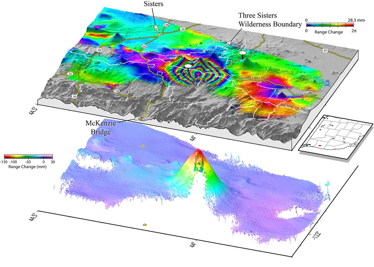
In 1997 the ground of a wilderness in the Cascade Range, near the cluster of volcanoes called the Three Sisters, began to rise. By 2001 its centre stood $15\,\mathrm{cm}$ higher. No volcano stands directly above the swelling, and the last eruption in the area was 1,500 years old. The uplift was not found by anyone walking on it: it appeared as a bull’s eye of coloured rings when radar images of the region, taken from orbit years apart, were combined. The rings placed the intruding magma 6 to $7\,\mathrm{km}$ down; in March 2004 a swarm of more than 300 small earthquakes struck next to their centre. This chapter explains how a satellite measures a change of a few centimetres from hundreds of kilometres up, what the other sensors in orbit see of the ground, and how the maps they make are combined in a geographic information system.

You already know

The electromagnetic spectrum, Planck’s law of the black body, emissivity and Kirchhoff’s law, reflectance and the interference of waves are in the physics books. Remote sensing, satellite images, map projections and satellite positioning are in the school books. Atmospheric windows and photometric bands are in the Year 1 volume, in its chapter on telescopes; the digital elevation model and the geographic information system that stores it, in its chapter on geological maps; the first radar map of an earthquake’s displacement, in its chapter on the earthquake source. The Mogi source of an inflating magma reservoir is in the Year 2 volume, in its chapter on volcanic eruptions.

25.1 Spectral signatures and optical sensors

Sunlight that reaches the ground is partly absorbed and partly reflected, in proportions that depend on the wavelength and on what the ground is made of. A sensor in orbit measures the reflected light in a few ranges of wavelength, its bands, and the ratios between the bands identify the surface.

Definition 25.1 (Spectral signature)

The spectral signature of a material is its reflectance as a function of wavelength, $R(\lambda)$, the fraction of the incident radiation it reflects. Over the thermal infrared, where surfaces emit rather than reflect, the signature is the emissivity $\varepsilon(\lambda)$; for an opaque sample $\varepsilon = 1 - R$.

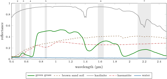
The signatures in the figure above are the vocabulary of optical remote sensing. The chlorophyll of leaves absorbs strongly between 0.4 and $0.7\,\text{µ}\mathrm{m}$, for photosynthesis, while the cells of the leaves reflect strongly between 0.7 and $1.1\,\text{µ}\mathrm{m}$: green grass reflects $5\,\%$ of the red light of band 4 and $50\,\%$ of the near infrared of band 5, a jump no rock or soil makes. Beyond, two deep dips near 1.4 and $1.9\,\text{µ}\mathrm{m}$ are where liquid water absorbs. The brown sand brightens steadily towards the infrared. Kaolinite, a clay, is white in the visible and has a narrow absorption at $2.20\,\text{µ}\mathrm{m}$, inside band 7, which makes it darker there than in band 6; a hyperspectral sensor resolves its shape and tells one clay from another. Haematite absorbs the blue and green: hence its red.

Definition 25.2 (Spatial, spectral and radiometric resolution; revisit time)

The spatial resolution of an image is the size on the ground of one of its pixels. Its spectral resolution is the number and width of its bands, its radiometric resolution the number of levels in which each measurement is recorded, $2^b$ for $b$ bits. The revisit time of a satellite is the interval between two of its observations of the same place.

The four cannot all be fine at once: smaller pixels and narrower bands collect less light each, and a narrow swath takes longer to cover the Earth. The imager of Landsat 8, launched in 2013, has nine bands, most of them with $30\,\mathrm{m}$ pixels and one panchromatic band at $15\,\mathrm{m}$; it records 4096 levels (12 bits) where the instruments of Landsats 1 to 7 recorded 256. From a sun-synchronous orbit $705\,\mathrm{km}$ up it images a swath $185\,\mathrm{km}$ wide and returns over the same ground every 16 days; Landsat 9, in the same orbit 8 days apart, halves the wait. The multispectral imager of each Sentinel-2 satellite has 13 bands, at 10, 20 or $60\,\mathrm{m}$, over a swath of $290\,\mathrm{km}$; with two satellites in the same orbit the revisit at the Equator is 5 days.

Definition 25.3 (Multispectral and hyperspectral sensors)

A multispectral sensor records a few to a few tens of bands, separated by gaps. A hyperspectral sensor records many narrow, contiguous bands, so that every pixel carries a nearly continuous spectrum that can be compared with a library such as the one of the figure above.

Between the ground and the sensor lies the atmosphere. It scatters sunlight into the sensor that never touched the ground, most of all at short wavelengths, the path radiance, and it absorbs part of what the ground reflects outside the windows.

Definition 25.4 (Atmospheric correction)

Atmospheric correction is the conversion of the radiance measured at the top of the atmosphere into the reflectance of the surface, by removing the path radiance and compensating the absorption along the two paths of the light, down and up.

The simplest correction subtracts in each band the value of the darkest pixels of the scene, deep clear water or a shadow, which should reflect nearly nothing: what they show is the path radiance. Careful corrections model the atmosphere’s molecules, aerosols and water vapour.

Definition 25.5 (Normalised difference vegetation index)

The normalised difference vegetation index (NDVI) of a pixel is

$$\mathrm{NDVI} = \frac{R_\mathrm{NIR} - R_\mathrm{red}}{R_\mathrm{NIR} + R_\mathrm{red}} ,$$

computed from its reflectances in a near-infrared and a red band.

The index lies between $-1$ and $+1$. Ground without green leaves gives a value close to zero, barren rock, sand or snow $0.1$ and below, shrubs and grassland 0.2 to 0.3, temperate and tropical rainforests 0.6 to 0.8; the densest green leaves approach 0.8 to 0.9. From the spectra of the figure above, through bands 4 and 5, the grass gives 0.82, the brown sand 0.15 and the water $-0.01$. Being a ratio, the index does not change when both bands are dimmed in the same proportion, by a slope facing away from the light or a thin uniform haze: it measures the vegetation, not the illumination. An additive path radiance, larger in the red, does change it, which is why the index is computed from corrected reflectances (Exercise 25.12).

25.2 The thermal infrared

At the temperatures of the ground, around $300\,\mathrm{K}$, Planck’s law puts the peak of a black body’s emission near $9.7\,\text{µ}\mathrm{m}$, in the atmospheric window of the thermal infrared. There the sensor measures what the surface emits, not what it reflects. The thermal sensor of Landsat 8 has two bands, 10.6 to 11.19 and 11.5 to $12.51\,\text{µ}\mathrm{m}$, with $100\,\mathrm{m}$ pixels.

Definition 25.6 (Brightness temperature)

The brightness temperature $T_b$ of a surface at the wavelength $\lambda$ is the temperature of the black body that would emit the spectral radiance $L$ measured from it at that wavelength. The kinetic temperature is the surface’s thermodynamic temperature, the one a thermometer would read.

Proposition 25.7 (Brightness temperature from a radiance)

With $c_1 = 2hc^2$ and $c_2 = hc/k$, a spectral radiance $L$ at the wavelength $\lambda$ has the brightness temperature

$$T_b = \frac{c_2}{\lambda \ln\!\left(1 + \dfrac{c_1}{\lambda^5 L}\right)} .$$

A surface of emissivity $\varepsilon < 1$ at the kinetic temperature $T$ emits $L = \varepsilon B_\lambda(T)$ and has $T_b < T$.

The difference matters. At the centre of band 10, $10.9\,\text{µ}\mathrm{m}$, a surface at $300\,\mathrm{K}$ with an emissivity of 0.95 has a brightness temperature of $296.6\,\mathrm{K}$, one of 0.99 $299.3\,\mathrm{K}$: a percent of emissivity is worth more than half a kelvin. The laboratory spectra give, in band 10, an emissivity of 0.98 for the grass, 0.99 for the water and 0.97 for the brown sand. Mapping a temperature from orbit therefore needs the emissivity of every pixel, and a correction for the emission and the absorption of the air between.

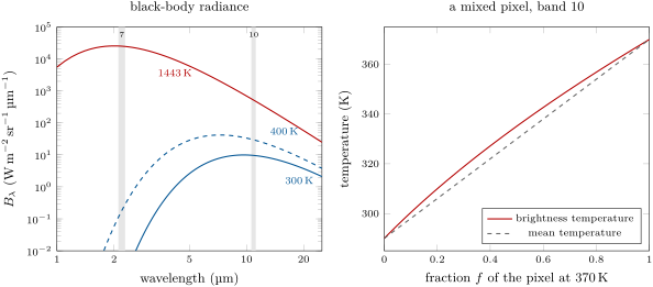
Lava at $1170\,{}^{\circ}\mathrm{C}$ has its peak near $2.0\,\text{µ}\mathrm{m}$: a fresh lava flow far smaller than a pixel lights up the shortwave infrared bands of an optical imager, by day or night. A pixel is rarely uniform, and Planck’s law is not linear in the temperature.

Proposition 25.8 (A mixed pixel)

A pixel of which a fraction $f$ emits as a black body at $T_h$ and the rest at $T_0 < T_h$ has the radiance $L = fB_\lambda(T_h) + (1 - f)B_\lambda(T_0)$, and, for $0 < f < 1$, its brightness temperature exceeds the area-weighted mean temperature $fT_h + (1 - f)T_0$.

A pixel with $5\,\%$ of fumarole ground at $370\,\mathrm{K}$ in a background at $290\,\mathrm{K}$ has a mean temperature of $294\,\mathrm{K}$ but a brightness temperature of $295.3\,\mathrm{K}$; at $10\,\%$, $300.4\,\mathrm{K}$. Hot spots stand out of a thermal image, and their temperature cannot be read from one band alone: two bands of different wavelength give two equations for $f$ and $T_h$.

25.3 Radar and lidar

An optical or thermal sensor is passive: it measures the light the ground sends. A radar or a lidar is active: it sends a pulse and times its echo. Microwaves pass through clouds, and the radar brings its own illumination, so it observes by day and night in any weather.

Definition 25.9 (Synthetic-aperture radar; radar backscatter)

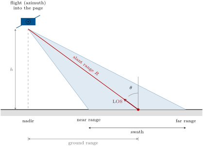
A synthetic-aperture radar (SAR) is a radar carried along a track that looks sideways, and that combines the echoes it records from the same point of the ground along a length of its track, keeping their phases, as if they had been received by one antenna as long as that length. The radar backscatter of a surface is the fraction of the power it receives that it sends back towards the antenna.

Proposition 25.10 (Azimuth resolution)

A real antenna of length $L$ at the slant range $R$ separates two points of the ground along its track only if they are more than about $R\lambda/L$ apart. A synthetic-aperture radar with the same antenna reaches about $L/2$, whatever the range.

The radar of each Sentinel-1 satellite works in the C band, at $5.405\,\mathrm{GHz}$, a wavelength of about $5.55\,\mathrm{cm}$, with an antenna $12.3\,\mathrm{m}$ long, from $693\,\mathrm{km}$ up. A real antenna that size would see details no finer than about $4\,\mathrm{km}$ along the track; the synthetic aperture brings $L/2$ to about $6\,\mathrm{m}$. Over land it works mostly in a wide-swath mode that scans three sub-swaths to cover $250\,\mathrm{km}$, at incidence angles between 29 and $46{}^{\circ}$, with cells of 5 by $20\,\mathrm{m}$. One satellite repeats its orbit every 12 days.

The backscatter depends on the roughness of the surface at the scale of the wavelength and on its moisture. A calm lake reflects the pulse away, like a mirror, and is black; a rough lava flow, a forest canopy or a city of walls and corners sends much of it back and is bright.

Definition 25.11 (Lidar)

A lidar measures distances by the travel time of laser pulses reflected by the ground, the vegetation or the water.

Proposition 25.12 (Time of flight)

A pulse that returns a time $t$ after it left has met a surface at the distance $ct/2$; an uncertainty $\delta t$ on the time is an uncertainty $c\,\delta t/2$ on the distance.

The laser altimeter of ICESat-2, about $500\,\mathrm{km}$ up, fires $10\,000$ pulses a second at $532\,\mathrm{nm}$ in six beams, one every $0.7\,\mathrm{m}$ along the ground in a footprint $11\,\mathrm{m}$ across. Of the about 300 trillion photons that leave with each pulse only about a dozen return, and each is timed to $800\,\mathrm{ps}$: $12\,\mathrm{cm}$ of range. Over a forest some photons return from the canopy and some from the ground through its gaps: the difference is the height of the trees, and the ground photons alone give a map of the relief beneath. Lidars flown on aircraft map the ground under the vegetation the same way.

25.4 Radar interferometry

The echo recorded by a radar has an amplitude, the strength of the return, and a phase, which counts the round-trip distance in units of the wavelength. The phase of one image alone is useless: each pixel holds many scatterers whose echoes add with random phases. But if the ground does not change in between, the same scatterers give the same sum again.

Definition 25.13 (Radar interferometry; interferogram; line of sight)

Radar interferometry (InSAR) combines two radar images of the same ground, taken from nearly the same position at two times, pixel by pixel. Their interferogram is the map of the difference of their phases, known modulo $2\pi$ and drawn as a cycle of colours, one cycle a fringe. The line of sight is the direction from the ground to the antenna; the radar measures only the component of a displacement along it. Phase unwrapping is the reconstruction of the continuous phase from the wrapped one, by adding to each pixel the multiple of $2\pi$ that makes the phase vary smoothly from its neighbours.

Theorem 25.14 (One fringe)

Between two acquisitions from the same position, a displacement of the ground that shortens the distance to the antenna by $\Delta r$ changes the phase of its echo by $\Delta\phi = 4\pi\Delta r/\lambda$. One fringe, a change of $2\pi$, is a motion of $\lambda/2$ along the line of sight.

For Sentinel-1 a fringe is $27.7\,\mathrm{mm}$; for the older European and Canadian satellites, of wavelength $5.66\,\mathrm{cm}$, $28.3\,\mathrm{mm}$, the cycle of colours of the photograph below. In practice the positions of the two passes differ, by up to a hundred metres or so (Sentinel-1 is held within $120\,\mathrm{m}$ of a reference orbit), and the phase difference also contains the relief, which a digital elevation model removes; the atmosphere’s water vapour delays the waves differently on the two dates; and where the ground changes between the passes, vegetation above all, the phases lose their coherence and the fringes dissolve into noise. The longer L-band wavelength, $23.53\,\mathrm{cm}$, sees through vegetation better than the C band.

Proposition 25.15 (A Mogi source seen along the line of sight)

Above a Mogi source of volume change $\Delta V$ at depth $z_0$, at the horizontal distance $r$, the ground moves up by $u_z$, as in the Year 2 volume, and outwards by

$$u_r = \frac{(1 - \nu)\,\Delta V}{\pi}\,\frac{r}{(r^2 + z_0^2)^{3/2}} = \frac{r}{z_0}\,u_z .$$

Seen at the incidence $\theta$ from a satellite to the east, the change of the line of sight is $d = u_E\sin\theta + u_z\cos\theta$, $u_E$ the eastward displacement. Along the north–south line through the centre, $d = u_z\cos\theta$.

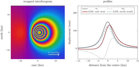
The fringes are counted from a part of the image that did not move. Their number gives the motion at the centre; the width of the pattern gives the depth, as for the uplift profile in the Year 2 volume, along the north–south line where the horizontal motion is invisible to the radar. The first such map, of the displacement of a large Californian earthquake in 1992, appeared in the Year 1 volume; since then interferograms have mapped the slip of earthquakes, the subsidence of basins whose aquifers are pumped, $3\,\mathrm{cm}$ over some $8\,\mathrm{km}$ in one Californian valley in 1997, and the swelling of volcanoes such as the Three Sisters.

In the lab — A ground station

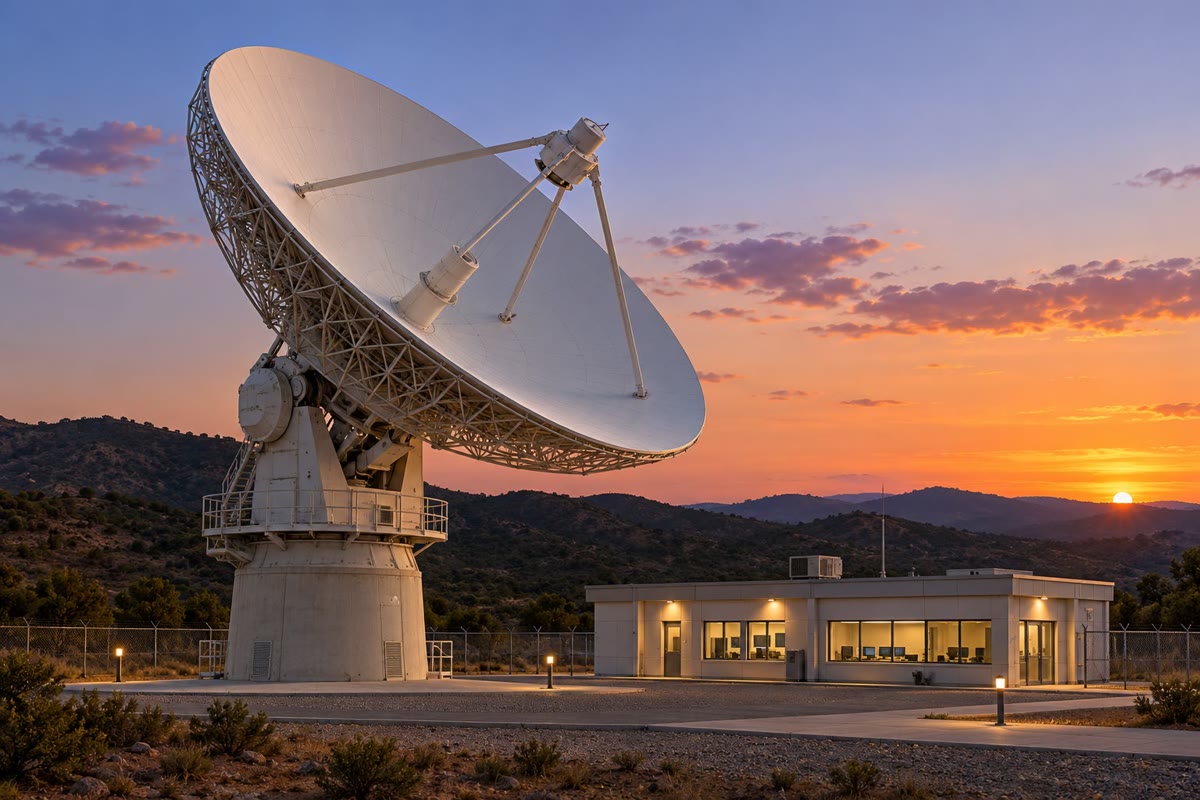
An imaging satellite records far more than it can send while it passes over the place it images. The radar of a Sentinel-1 satellite can image for up to half an hour of each orbit and stores its data on board, up to 1410 gigabits; it sends them down over two channels of 260 megabits a second each, so a full store takes some 45 minutes to empty. A ground station receives them: as the satellite rises above the horizon, the dish turns to point at it, follows it across the sky and lets it go as it sets, while the operators check that the stream arrives complete. The data then go to a processing centre, where the raw echoes become images.

25.5 Geographic information systems

The images of the satellites, the elevation model of the ground, the geological map, the wells and the roads are layers of one geographic information system, which stores them in a common frame of coordinates and computes with them.

Definition 25.16 (Raster and vector data)

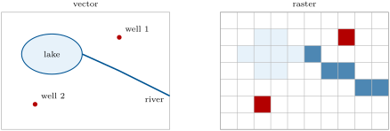
Raster data represent a layer by a grid of cells, each holding one value: a reflectance, an elevation, a class. Vector data represent it by points, lines and polygons given by the coordinates of their vertices, each carrying a row of attributes in a table.

Definition 25.17 (Georeferencing)

Georeferencing is the assignment of map coordinates in a stated projection to every pixel of an image or every vertex of a drawing, usually by fitting a transformation to ground control points whose positions are known in both.

For a north-up raster in a projected frame the transformation is affine: the cell in column $i$ and row $j$ has its corner at $E = E_0 + i\,\Delta$, $N = N_0 - j\,\Delta$, with $\Delta$ the cell size. A satellite image is first resampled into such a grid; layers in different projections are projected into one before they are combined.

Method 25.18 (Slope, aspect and hillshade from a digital elevation model)

On a grid of elevations $z_{i,j}$ of spacing $\Delta$ ($i$ eastward, $j$ northward), estimate the gradient by central differences,

$$\frac{\partial z}{\partial x} \approx \frac{z_{i+1,j} - z_{i-1,j}}{2\Delta} , \qquad \frac{\partial z}{\partial y} \approx \frac{z_{i,j+1} - z_{i,j-1}}{2\Delta} .$$

The slope is $S = \arctan|\nabla z|$; the aspect is the azimuth of steepest descent, the direction of $-\nabla z$, $A = \operatorname{atan2}(-\partial z/\partial x, -\partial z/\partial y)$ measured clockwise from north. The hillshade for a light from the azimuth $A_0$ at the zenith angle $Z$ is $\cos Z\cos S + \sin Z\sin S \cos(A_0 - A)$, the cosine of the angle between the light and the normal to the ground, set to zero where it is negative.

The central difference is exact for a plane and in error by $\Delta^2 z'''/6$ otherwise; the shaded relief of the Varden Hills in the Year 1 volume was computed this way, lit from the north-west. Derivatives amplify the errors of the grid: a model with steps between its rows shows them as stripes in its slope map.

Definition 25.19 (Map algebra)

Map algebra is the computation of a new raster layer cell by cell from one or more layers of the same grid: by arithmetic (the NDVI from two bands), by comparison (the cells steeper than $15{}^{\circ}$), by logical operations (and, or, not), or from a neighbourhood of the cell (the slope).

Definition 25.20 (Buffer; overlay)

The buffer of a feature at the distance $d$ is the region of the map within $d$ of it. An overlay combines two or more layers of the same area into one, each place of the result carrying the attributes of all of them; the selection of the places that meet several conditions at once is the commonest use.

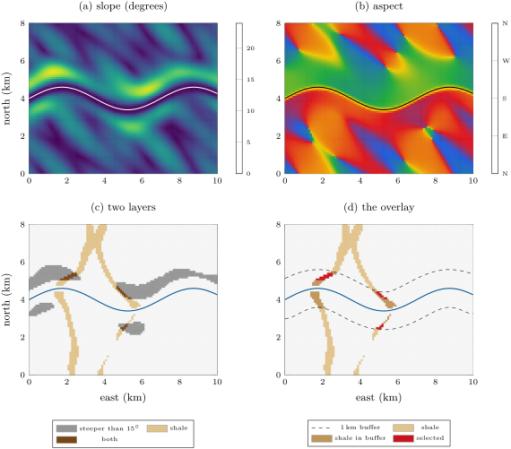
The figure above runs the whole chain: map algebra on the elevation grid gives the slope and the aspect; a comparison turns the slope into a layer of steep cells; the geological map gives the shale; the buffer of the river gives a third layer; their intersection, an overlay with the logical and, leaves 32 cells of the 8181. The answer is only as good as the layers: on a coarser grid the slopes come out gentler and fewer cells pass.

Definition 25.21 (Supervised classification; confusion matrix)

A supervised classification assigns each pixel of an image to one of a set of classes, from rules or statistics learned on training pixels whose class is known on the ground. Its confusion matrix counts, for a separate set of reference pixels, how many of each true class were assigned to each class: $n_{ij}$ pixels classified as $i$ belong in truth to $j$.

The diagonal holds the pixels classified right. With $N$ reference pixels, the overall accuracy is $\sum_i n_{ii}/N$. The user’s accuracy of a class, $n_{ii}$ over its row total, is the chance that a pixel the map calls $i$ is $i$; its producer’s accuracy, $n_{ii}$ over its column total, the chance that a true $i$ was mapped as $i$. The kappa coefficient compares the overall accuracy $p_o$ with the accuracy $p_e = \sum_i (\text{row}_i)(\text{col}_i)/N^2$ that random assignment with the same totals would reach: $\kappa = (p_o - p_e)/(1 - p_e)$.

In this invented example, 113 of 130 pixels are right, an overall accuracy of $86.9\,\%$. Forest has a user’s accuracy of $38/48 = 79\,\%$ but a producer’s accuracy of $38/45 = 84\,\%$: seven pixels of bare rock, perhaps in shadow, were called forest. Random assignment would reach $p_e = 0.338$, and $\kappa = 0.80$.

25.6 Exercises

Exercise 25.1 ★

A field has reflectances of 0.06 in the red band and 0.42 in the near-infrared band of an imager; a ploughed field next to it 0.21 and 0.28. Compute the NDVI of both and say what each value suggests.

Solution

Solution of Exercise 25.1.

Field: $(0.42 - 0.06)/(0.42 + 0.06) = 0.75$, dense green vegetation, a crop in full leaf. Ploughed field: $(0.28 - 0.21)/(0.28 + 0.21) = 0.14$, nearly bare ground, a soil that brightens slightly towards the infrared.

Exercise 25.2 ★

The Landsat 8 imager covers a swath $185\,\mathrm{km}$ wide with $30\,\mathrm{m}$ pixels, and its panchromatic band with $15\,\mathrm{m}$ pixels. (a) How many pixels does a line across the swath hold in each case? (b) How many levels do 12 bits give, and 8 bits? (c) What is the revisit time of Landsat 8 alone, and of Landsats 8 and 9 together?

Solution

Solution of Exercise 25.2.

(a) $185000/30 \approx 6170$ pixels; $185000/15 \approx 12300$ in the panchromatic band. (b) $2^{12} = 4096$ levels; $2^8 = 256$. (c) 16 days alone; with Landsat 9 in the same orbit 8 days apart, 8 days.

Exercise 25.3 ★

(a) On a Sentinel-1 interferogram ($\lambda = 5.55\,\mathrm{cm}$) of a subsiding basin, six fringes separate the stable edge from the centre. What is the change of the line of sight at the centre? (b) What would one fringe be for an older satellite of wavelength $5.66\,\mathrm{cm}$?

Solution

Solution of Exercise 25.3.

(a) One fringe is $\lambda/2 = 27.7\,\mathrm{mm}$; six fringes are $166\,\mathrm{mm}$ of line-of-sight change, here away from the satellite, since the basin subsides. (b) $56.6/2 = 28.3\,\mathrm{mm}$.

Exercise 25.4 ★

A laser altimeter is $500\,\mathrm{km}$ above the ground. (a) How long does a pulse take to return? (b) If each photon is timed to $800\,\mathrm{ps}$, how precise is one range?

Solution

Solution of Exercise 25.4.

(a) $t = 2d/c = 2\times5 \times 10^{5}/3.00 \times 10^{8} = 3.34\,\mathrm{ms}$. (b) $c\,\delta t/2 = 3.00 \times 10^{8}\times8 \times 10^{-10}/2 = 0.12\,\mathrm{m}$; a surface sampled by many photons is located much better, the precision falling as one over the square root of their number.

Exercise 25.5 ★★

A pixel of Landsat 8’s band 10 (take $\lambda = 10.9\,\text{µ}\mathrm{m}$) has, after atmospheric correction, a spectral radiance of $9.0\,\mathrm{W}\,\mathrm{m}^{-2}\,\mathrm{sr}^{-1}\,\text{µ}\mathrm{m}^{-1}$. (a) Compute its brightness temperature. (b) The surface is a grass field of emissivity 0.98: what is its kinetic temperature?

Solution

Solution of Exercise 25.5.

(a) In SI units $L = 9.0 \times 10^{6}\,\mathrm{W}\,\mathrm{m}^{-2}\,\mathrm{sr}^{-1}\,\mathrm{m}^{-1}$. With $c_1 = 2hc^2 = 1.191 \times 10^{-16}\,\mathrm{W}\,\mathrm{m}^{2}\,\mathrm{sr}^{-1}$, $c_2 = 0.014\,388\,\mathrm{m}\,\mathrm{K}$ and $\lambda^5 = (1.09 \times 10^{-5})^5 = 1.539 \times 10^{-25}$, $c_1/(\lambda^5L) = 86.0$, and $T_b = c_2/(\lambda\ln 87.0) = 295.6\,\mathrm{K}$. (b) The kinetic temperature solves $0.98\,B_\lambda(T) = L$, that is $B_\lambda(T) = L/0.98$: the same formula gives $T = 296.9\,\mathrm{K}$, $1.3\,\mathrm{K}$ more.

Exercise 25.6 ★★

The Sentinel-1 radar flies $693\,\mathrm{km}$ up with an antenna $12.3\,\mathrm{m}$ long at $\lambda = 5.55\,\mathrm{cm}$. (a) Ignoring the curvature of the Earth, compute the slant range to a point seen at an incidence of $35{}^{\circ}$. (b) What azimuth resolution would a real antenna of that length give there, and what does the synthetic aperture give? (c) How long is the synthetic aperture?

Solution

Solution of Exercise 25.6.

(a) $R = 693/\cos35{}^{\circ} = 846\,\mathrm{km}$. (b) Real antenna: $R\lambda/L = 8.46 \times 10^{5}\times0.0555/12.3 = 3.8\,\mathrm{km}$; synthetic aperture: $L/2 = 6.2\,\mathrm{m}$, some 600 times finer. (c) The synthetic aperture is the length of track over which a point stays in the beam, $R\lambda/L = 3.8\,\mathrm{km}$.

Exercise 25.7 ★★

A $3\times3$ window of a digital elevation model with $30\,\mathrm{m}$ cells reads, north at the top,

$$\begin{matrix} 412 & 418 & 425 \\ 405 & 410 & 418 \\ 398 & 401 & 409 \end{matrix} \qquad (\mathrm{m}).$$

By central differences at the centre cell, compute the slope, the aspect and the hillshade for a light from the north-west, $45{}^{\circ}$ above the horizon.

Solution

Solution of Exercise 25.7.

$\partial z/\partial x = (418 - 405)/60 = 0.217$ (east minus west), $\partial z/\partial y = (418 - 401)/60 = 0.283$ (north minus south); $|\nabla z| = 0.357$, a slope of $\arctan 0.357 = 19.6{}^{\circ}$. The ground rises to the north-east, so it faces the south-west: $A = \operatorname{atan2}(-0.217, -0.283) = 217{}^{\circ}$. Hillshade: $\cos45{}^{\circ} \cos19.6{}^{\circ} + \sin45{}^{\circ}\sin19.6{}^{\circ}\cos(315{}^{\circ} - 217{}^{\circ}) = 0.666 - 0.033 = 0.63$, a little darker than flat ground (0.71): the slope turns slightly away from a light in the north-west.

Exercise 25.8 ★★

A land-cover map is checked against 160 reference pixels (rows: the map; columns: the truth; classes water, forest, crops, town):

$$\begin{pmatrix} 48 & 3 & 1 & 0 \\ 4 & 37 & 6 & 1 \\ 2 & 5 & 29 & 2 \\ 0 & 1 & 2 & 19 \end{pmatrix} .$$

Compute the overall accuracy, the user’s and producer’s accuracies of each class, and kappa. Which class is most often missed?

Solution

Solution of Exercise 25.8.

Row totals 52, 48, 38, 22; column totals 54, 46, 38, 22; diagonal 133 of 160: overall accuracy $83.1\,\%$. User’s accuracies: water $48/52 = 0.92$, forest $37/48 = 0.77$, crops $29/38 = 0.76$, town $19/22 = 0.86$. Producer’s: water $48/54 = 0.89$, forest $37/46 = 0.80$, crops $29/38 = 0.76$, town $19/22 = 0.86$. $p_e = (52\cdot54 + 48\cdot46 + 38\cdot38 + 22\cdot22)/160^2 = 0.271$, $\kappa = (0.831 - 0.271)/(1 - 0.271) = 0.77$. Crops are most often missed: 9 of the 38 true crop pixels went elsewhere, mostly to forest.

Exercise 25.9 ★★

A $100\,\mathrm{m}$ thermal pixel contains a fresh lava flow at $1443\,\mathrm{K}$ covering $4\,\%$ of it; the rest is ground at $290\,\mathrm{K}$; take both as black bodies. (a) Compute the brightness temperature of the pixel at $10.9\,\text{µ}\mathrm{m}$ and compare it with the mean temperature. (b) Compute the ratio of the black-body radiances of the lava and the ground at $2.2\,\text{µ}\mathrm{m}$, and the brightness temperature of the pixel there. Which band detects the lava better?

Solution

Solution of Exercise 25.9.

(a) $L = 0.04\,B_\lambda(1443) + 0.96\,B_\lambda(290)$ at $10.9\,\text{µ}\mathrm{m}$, $28.6\,\mathrm{W}\,\mathrm{m}^{-2}\,\mathrm{sr}^{-1}\,\text{µ}\mathrm{m}^{-1}$, whose brightness temperature is $396\,\mathrm{K}$, against a mean temperature of $0.04\times1443 + 0.96\times290 = 336\,\mathrm{K}$. (b) At $2.2\,\text{µ}\mathrm{m}$, $B_\lambda(1443)/B_\lambda(290) = 6.8 \times 10^{7}$: the lava dominates the pixel completely, and its brightness temperature is $845\,\mathrm{K}$. The shortwave infrared band detects small hot spots far better; the thermal band, sensitive to the whole pixel, is the one that measures the ground around them.

Exercise 25.10 ★★★

Two interferograms of the same deformation are made from two passes, one with the satellite to the east of the ground and one with it to the west, both at an incidence of $35{}^{\circ}$. At one point the line of sight shortens by $64\,\mathrm{mm}$ on the first and $38\,\mathrm{mm}$ on the second. Assuming no north–south motion, compute the vertical and the eastward displacements. Why is one pass not enough?

Solution

Solution of Exercise 25.10.

With the satellite to the east, $d_1 = u_E\sin\theta + u_z\cos\theta$; to the west, $d_2 = -u_E\sin\theta + u_z\cos\theta$. Adding and subtracting, $u_z = (d_1 + d_2)/(2\cos\theta) = 102/1.638 = 62.3\,\mathrm{mm}$ and $u_E = (d_1 - d_2)/(2\sin\theta) = 26/1.147 = 22.7\,\mathrm{mm}$. One pass gives one equation for two unknowns: any mixture of uplift and eastward motion with the same projection on the line of sight gives the same fringes.

Exercise 25.11 ★★★

Unwrapping fails where the phase jumps by more than $\pi$ between neighbouring pixels. (a) Show that the line of sight must change by less than $\lambda/4$ from one pixel to the next, $13.9\,\mathrm{mm}$ for Sentinel-1. (b) For a Mogi source at $z_0 = 4\,\mathrm{km}$ with $\Delta V = 10^{7}\,\mathrm{m}^{3}$ and $\nu = 0.25$, seen vertically, show that the steepest gradient of $u_z$ is at $r = z_0/2$ and compute it. (c) What is the largest pixel size that keeps the fringes resolvable?

Solution

Solution of Exercise 25.11.

(a) By Theorem 25.14, $\Delta\phi = 4\pi\Delta r/\lambda < \pi$ requires $\Delta r < \lambda/4 = 13.9\,\mathrm{mm}$. (b) $u_z = k z_0(r^2 + z_0^2)^{-3/2}$ with $k = (1 - \nu)\Delta V/\pi$; $\mathrm du_z/\mathrm dr = -3kz_0r(r^2 + z_0^2)^{-5/2}$, whose derivative vanishes where $(r^2 + z_0^2) = 5r^2$, at $r = z_0/2$. There

$$\left|\frac{\mathrm du_z}{\mathrm dr}\right| = \frac{3k}{2z_0^3}\Big(\frac54\Big)^{-5/2} = \frac{0.859\,k}{z_0^3} = \frac{0.859\times2.39 \times 10^{6}}{6.4 \times 10^{10}} = 3.2 \times 10^{-5},$$

$32\,\mathrm{mm}$ per kilometre. (c) $13.9/32 = 0.43\,\mathrm{km}$: pixels smaller than about $430\,\mathrm{m}$, easily met by Sentinel-1’s.

Exercise 25.12 ★★★

(a) Show that the NDVI lies between $-1$ and $+1$ for non-negative reflectances, and that it is unchanged when both reflectances are multiplied by the same factor. (b) Grass has reflectances of 0.051 (red) and 0.502 (near infrared). An uncorrected image adds a path radiance equivalent to 0.03 in the red and 0.01 in the near infrared. Compute the NDVI with and without it. (c) What does that imply for a map of the NDVI made from uncorrected images on a hazy day?

Solution

Solution of Exercise 25.12.

(a) For $N, R \ge 0$ not both zero, $|N - R| \le N + R$, so $|\mathrm{NDVI}| \le 1$; replacing $N$ and $R$ by $aN$ and $aR$ multiplies the numerator and the denominator by $a$. (b) Without: $(0.502 - 0.051)/(0.502 + 0.051) = 0.816$; with: $(0.512 - 0.081)/(0.512 + 0.081) = 0.727$. (c) The path radiance lowers the index of green vegetation, by about a tenth here, and by an amount that changes with the haze: a map of uncorrected images would show the weather as much as the vegetation, and comparisons between dates would be meaningless.

25.7 Problem: A Swelling Flank at Mount Halvren

Problem 25.1

Weekend problem — vegetation, heat and a radar interferogram on an invented volcano

Mount Halvren, an invented volcano, has erupted lava flows in 1890, 1960 and 2005 onto its forested flanks. A fumarole field steams on its summit. Satellite data of a recent year are given below.

Part I — Vegetation on the lava flows. Corrected reflectances in the red and near-infrared bands:

surface	forest	flow of 1890	flow of 1960	flow of 2005
red	0.04	0.07	0.11	0.12
near infrared	0.38	0.30	0.21	0.14

1. Compute the NDVI of the four surfaces.
2. Rank the flows by the recovery of their vegetation. Is the ranking that of their ages?
3. Why is the NDVI of the flow of 2005 not zero, although almost nothing grows on it?
4. Why is the NDVI more reliable than the near-infrared reflectance alone on the steep, unevenly lit flanks of a volcano?

Part II — The fumarole field. In the thermal band (take $\lambda = 10.9\,\text{µ}\mathrm{m}$) the corrected radiance of a $100\,\mathrm{m}$ pixel of the summit plateau away from the fumaroles is $8.40\,\mathrm{W}\,\mathrm{m}^{-2}\,\mathrm{sr}^{-1}\,\text{µ}\mathrm{m}^{-1}$, and that of the pixel over the fumarole field $9.95\,\mathrm{W}\,\mathrm{m}^{-2}\,\mathrm{sr}^{-1}\,\text{µ}\mathrm{m}^{-1}$.

5. Compute the brightness temperatures of the two pixels.
6. The plateau’s rock has an emissivity of 0.97. What is its kinetic temperature?
7. The fumarole vents and the warm ground around them are at $370\,\mathrm{K}$. Treating them and the rest of the pixel as black bodies, the rest at the plateau’s radiance, what fraction of the pixel do they cover, and what area?
8. Why does the area-weighted mean temperature of the pixel fall short of its brightness temperature?

Part III — The interferogram. Two Sentinel-1 images ($\lambda = 5.55\,\mathrm{cm}$, incidence $35{}^{\circ}$, satellite to the east) taken 48 days apart show a bull’s eye on the east flank. From a stable area to the centre of the pattern one counts five full fringes and four tenths of a sixth, all of them in the sense of motion towards the satellite.

9. Why must two images be taken from nearly the same position, and how many orbital cycles of one satellite separate them?
10. Compute the change of the line of sight at the centre.
11. At the centre the ground moves only vertically. Compute the uplift there.
12. Explain why the pattern is not circular, and on which side, east or west, the fringes are crowded.
13. Along the north–south line through the centre, the change of the line of sight falls to half its central value $3.4\,\mathrm{km}$ from the centre. Why use that line, and what depth does it give for a Mogi source?
14. How many fringes separate the centre from that half-height point?
15. Water vapour in the air can delay the radar waves differently on the two dates and draw fringes of its own. How would a second interferogram, of another pair of dates, help tell the two apart?

Part IV — The volume. Take $\nu = 0.25$.

16. From $u_z(0) = (1 - \nu)\Delta V/(\pi z_0^2)$, compute the volume change of the source.
17. Express it as an average rate per day and per year over the 48 days.
18. Compute the largest horizontal displacement and where it occurs.
19. If the reservoir were a sphere of radius $z_0/3$, how large would its volume be, and what fraction of it does the change represent?
20. The finite size of a sphere of radius $z_0/3$ changes the uplift by about $3\,\%$. Does it change the answer of question 16 appreciably, given the precision of the fringe count?
21. What other observation, from Parts I and II or from the ground, would support the interpretation of a filling reservoir?
22. Give the volume change of the reservoir under Mount Halvren, in millions of cubic metres, to two significant figures.

Solution

Solution of Problem 25.1.

1. Forest $(0.38 - 0.04)/0.42 = 0.81$; flow of 1890 $0.23/0.37 = 0.62$; of 1960 $0.10/0.32 = 0.31$; of 2005 $0.02/0.26 = 0.08$.

2. 1890, then 1960, then 2005: the oldest flow is the greenest, in the order of the ages; it has not yet reached the forest.

3. Bare rock reflects slightly more in the near infrared than in the red, like the brown sand of the chapter’s figure; lichens and the first plants add a little: 0.08 is the value of nearly bare ground.

4. A slope turned away from the light dims both bands in the same proportion; the ratio cancels it, while the near-infrared reflectance alone would mistake a shaded forest for sparse vegetation.

5. By Proposition 25.7 with $\lambda = 10.9\,\text{µ}\mathrm{m}$: the plateau $291.1\,\mathrm{K}$, the fumarole pixel $302.3\,\mathrm{K}$.

6. $0.97\,B_\lambda(T) = 8.40 \times 10^{6}$ gives $T = 293.0\,\mathrm{K}$.

7. $B_\lambda(370\,\mathrm{K}) = 22.48\,\mathrm{W}\,\mathrm{m}^{-2}\,\mathrm{sr}^{-1}\,\text{µ}\mathrm{m}^{-1}$; $f = (9.95 - 8.40)/(22.48 - 8.40) = 0.110$, about $1100\,\mathrm{m}^{2}$ of the $10^{4}\,\mathrm{m}^{2}$ pixel.

8. The radiance is a convex function of the temperature (Proposition 25.8): the hot part adds more radiance than its share of the temperature, so the pixel looks hotter than its mean, $0.110\times370 + 0.890\times291.1 = 299.8\,\mathrm{K}$ against $302.3\,\mathrm{K}$.

9. The phase of each echo depends on the exact path; a large change of viewpoint changes the sum of the scatterers’ echoes and the interferogram loses its coherence, and it adds a phase from the relief. $48/12 = 4$ cycles of one satellite.

10. $5.4\times27.73 = 149.7\,\mathrm{mm}$ towards the satellite.

11. $u_z = 149.7/\cos35{}^{\circ} = 182.8\,\mathrm{mm}$.

12. The ground moves outwards as well as up; on the east side the outward motion is towards the satellite and adds to the uplift, on the west side it subtracts (Proposition 25.15). The change falls faster to the west, where the fringes are crowded; the pattern is stretched to the east.

13. On that line the horizontal motion is north–south, perpendicular to the look, so the radar sees $u_z\cos\theta$ alone, of the shape of the uplift. The uplift halves at $r = 0.766\,z_0$, so $z_0 = 3.4/0.766 = 4.44\,\mathrm{km}$.

14. Half of 5.4: 2.7 fringes.

15. A deformation is the same on the two interferograms after scaling by the time intervals, or keeps growing from pair to pair; an atmospheric pattern changes from date to date and often follows the relief. A second pair that shows the same bull’s eye confirms the deformation.

16. $\Delta V = \pi u_z(0)z_0^2/(1 - \nu) = \pi\times0.1828\times 4436^2/0.75 = 1.51 \times 10^{7}\,\mathrm{m}^{3}$.

17. $1.51 \times 10^{7}/48 = 3.1 \times 10^{5}\,\mathrm{m}^{3}$ a day, $1.1 \times 10^{8}\,\mathrm{m}^{3}$ a year if the rate held.

18. $u_r \propto r/(r^2 + z_0^2)^{3/2}$ is largest where its derivative vanishes, $r^2 + z_0^2 = 3r^2$, $r = z_0/\sqrt2 = 3.14\,\mathrm{km}$; there $u_r = 70\,\mathrm{mm}$, $38\,\%$ of the central uplift.

19. Radius $1.48\,\mathrm{km}$, volume $\frac43\pi(1.48)^3 = 13.6\,\mathrm{km}^{3}$; the change is $1.51 \times 10^{7}/1.36 \times 10^{10} = 0.11\,\%$ of it.

20. No: a tenth of a fringe is $2\,\%$ of the count, and the depth, read from a half-width of $3.4\,\mathrm{km}$ perhaps to $0.1\,\mathrm{km}$, enters squared, $6\,\%$; the $3\,\%$ correction is within that uncertainty.

21. The warming of the fumarole field (Part II) over time, an increase in small earthquakes beneath the bulge, a change in the gas released, and uplift measured by satellite positioning or levelling at a few points of the flank.

22. The reservoir under Mount Halvren grew by 15 million $\mathrm{m}^{3}$ ($1.51 \times 10^{7}\,\mathrm{m}^{3}$).