18Quantitative Geomorphology

A river crossing a rising range has a step in its long profile: a waterfall, with a gorge below it and a gentler valley above. The step does not stay where it formed. It climbs upstream, a few millimetres or a few metres a year, and its position is a clock that started when the river’s base was lowered. Reading that clock, and the rates written in the shapes of hills and rivers, takes two conservation laws and two transport laws: one for the soil that creeps down a slope, one for the bedrock that a river cuts.

You already know

Weathering, erosion, deposition, landforms and the balance between uplift and erosion are in the school books, as are isostatic rebound and U-shaped glacial valleys. The denudation rate, the bed shear stress and the Shields parameter are in the Year 1 volume, in its chapter on erosion and transport; the digital elevation model in its chapter on geological maps; Airy isostasy in its chapter on isostasy and gravity anomalies. Cosmogenic nuclides and erosion rates from them are in Chapter 13, thermochronology and the age–elevation relationship in Chapter 10. The diffusion equation is in the physics books.

18.1 Hillslopes

On a soil-mantled hill, the soil moves downslope grain by grain: burrowing animals throw it, roots heave it, freezing and wetting swell it, and each disturbance lets gravity shift it a little. Averaged over centuries, the flux of soil is proportional to the slope.

Definition 18.1 (Hillslope diffusion)

Hillslope diffusion is the slow downslope transport of soil whose volume flux per unit width of slope, $\vec q$, is proportional to the gradient of the surface elevation $z$: $\vec q = -\kappa\,\nabla z$. The coefficient $\kappa$, in $\mathrm{m}^{2}/\mathrm{yr}$, is the hillslope diffusivity.

Theorem 18.2 (Diffusion of hillslopes)

Let rock be uplifted at a rate $U$ relative to the channels that bound a hillslope, soil and rock have the same density, and soil move by hillslope diffusion with uniform $\kappa$. Then the surface elevation obeys

$$\frac{\partial z}{\partial t} = U + \kappa\,\nabla^2 z ,$$

the diffusion equation with a source term.

A fault or a shoreline cuts a scarp at one moment; afterwards the scarp only diffuses. Starting from a vertical step of half-height $a$ on a far-field slope $b$, the solution in one dimension is

The shape depends only on the product $\kappa t$: a measured profile gives $\kappa t$, and either an independent age gives $\kappa$, or a known $\kappa$ gives the age, a morphological age. Scarps in semi-arid regions with granular soils and sparse vegetation give $\kappa$ between $10^{-3}$ and $10^{-2}\,\mathrm{m}^{2}/\mathrm{yr}$; humid, densely vegetated coastal mountains about $5 \times 10^{-3}\,\mathrm{m}^{2}/\mathrm{yr}$.

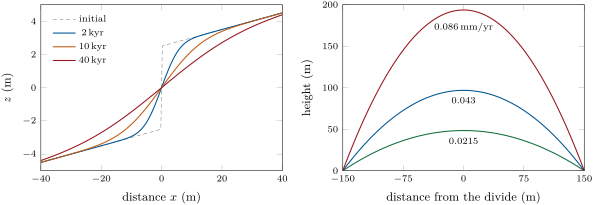
When a hill has been uplifted and eroded long enough, its shape stops changing: every point is lowered at the rate the rock rises.

Proposition 18.3 (Hilltop curvature gauges the erosion rate)

On a hillslope in steady state under hillslope diffusion, the erosion rate $E$, equal to $U$, is

$$E = -\kappa\,\nabla^2 z .$$

In one dimension the profile is the parabola $z = z_0 - E x^2/(2\kappa)$, with relief $E L^2/(2\kappa)$ between the divide and channels a distance $L$ away.

Curvature, a geometric quantity measured on a digital elevation model, thus reads as a rate once $\kappa$ is known: the steeper and more sharply rounded the hilltops, the faster the landscape erodes. The soil itself is made from the rock below at a rate that depends on how much soil already covers it.

Definition 18.4 (Soil production function)

The soil production function gives the rate $P$ at which bedrock is converted to soil as a function of the soil thickness $h$; it is commonly taken as $P = P_0\,e^{-h/h_0}$, where $P_0$ is the rate on bare rock and $h_0$ a length of a fraction of a metre.

At steady state the soil-rock interface is lowered at the rate of the surface, $P(h) = E$, so the soil thickness is $h = h_0 \ln(P_0/E)$: faster erosion means thinner soil, and where $E$ exceeds $P_0$ the soil is stripped and bare rock, limited by weathering, crops out. The fastest soil production rates measured are of the order of $0.5\,\mathrm{mm}/\mathrm{yr}$.

Linear diffusion fails on steep slopes. As the gradient approaches a threshold, grains roll and slide in bursts and shallow landslides strip the soil.

Definition 18.5 (Critical hillslope gradient)

The critical hillslope gradient $S_c$ is the gradient at which the soil flux grows without bound; in a widely used nonlinear transport law, $q = \kappa S/[1 - (S/S_c)^2]$.

Slopes much gentler than $S_c$ behave as in linear diffusion; slopes that erode fast steepen toward $S_c$ and become planar, their gradient set by the threshold rather than by the erosion rate.

In the field — Scanning a hillslope

A team surveying a soil-mantled ridge sets a terrestrial laser scanner on a tripod a few tens of metres from the crest. Each scan records millions of points, the distance and direction to the ground surface, through gaps in the grass and the shrubs; the points of several scan stations are merged into one cloud, registered to targets surveyed with a satellite receiver, and the last returns are kept to remove the vegetation. The bare-earth cloud is gridded into an elevation model of decimetre cells, smoothed over a few metres, and its Laplacian computed at the crest. The team then compares the hilltop curvatures of ridges eroding at rates measured with cosmogenic nuclides: plotted against each other, the two give the diffusivity of the hillslope as the slope of a line, as the proposition predicts.

18.2 River incision

Where a river runs on bedrock, it cuts down by plucking blocks, by abrasion under its bed load and by cavitation. All these scale with the shear stress the flow exerts on its bed, or the power it spends there, and both grow with discharge and slope. Discharge grows with drainage area, so area stands for discharge.

Definition 18.6 (Stream-power law)

The stream-power law gives the rate of vertical incision $E$ of a bedrock river as

$$E = K A^m S^n ,$$

where $A$ is the drainage area upstream of the point, $S$ the channel gradient, $m$ and $n$ positive exponents, and $K$ an erodibility coefficient that lumps rock strength, climate and channel width.

For processes that scale with shear stress or with unit stream power, $m/n$ is close to 0.5. A survey of badland channels cut in weak rock over about 20 years found incision rates proportional to $A^{0.44}S^{0.68}$.

Definition 18.7 (Detachment-limited and transport-limited incision)

Incision is detachment-limited when the river can carry away more sediment than it receives, so that its rate of lowering is set by how fast it detaches bedrock from its bed: the stream-power law applies. It is transport-limited when the river carries all the sediment it can, so that its bed is lowered only where the transport capacity grows downstream, at the rate set by the divergence of the sediment flux.

A transport-limited river behaves much like a hillslope: the flux depends on slope, and its profile evolves by a diffusion-like equation that rounds off any step. A detachment-limited river keeps a step sharp and moves it, as the next section shows. Mountain rivers with bedrock floors and thin gravel are usually closer to the first; rivers on thick alluvium to the second.

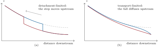
If rock rises at a uniform rate $U$ relative to the river’s outlet, and $K$, $m$, $n$ are uniform, the river evolves as $\partial z/\partial t = U - K A^m S^n$.

Definition 18.8 (Steady-state river profile)

A river profile is in steady state when its elevation no longer changes in time: at every point incision balances rock uplift relative to the outlet.

Theorem 18.9 (Steady-state profile under the stream-power law)

Under uniform $U$, $K$, $m$ and $n$, a detachment-limited river in steady state has the gradient

$$S = \left(\frac{U}{K}\right)^{1/n} A^{-m/n} .$$

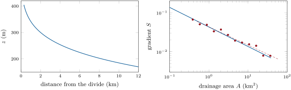
The gradient falls as a power of area: the profile is concave up. Real rivers follow such a power law even when the assumptions of the theorem are doubtful, so two numbers summarise a profile.

Definition 18.10 (Channel steepness and concavity indices)

When the gradient of a river follows $S = k_s A^{-\theta}$, the exponent $\theta$ is the concavity index and the coefficient $k_s$ the channel steepness index. To compare rivers, $\theta$ is set to a common reference value $\theta_{\mathrm{ref}}$, and $k_{sn} = S A^{\theta_{\mathrm{ref}}}$ is the normalised steepness.

By the theorem, $\theta = m/n$ and $k_s = (U/K)^{1/n}$: at a given erodibility, a river is steeper where rock rises faster. Steepness maps of a range therefore outline its uplift.

Gradients are derivatives of noisy elevations and scatter widely. Integrating the profile instead uses elevations, which are better measured.

Definition 18.11 (Chi analysis)

Chi analysis plots the elevation of the points of a river network against the coordinate

$$\chi(x) = \int_{x_b}^{x} \left(\frac{A_0}{A(x')}\right)^{\theta} \mathrm{d}x' ,$$

where $x$ is the distance upstream along the channel from a base point $x_b$, $A_0$ a reference area and $\theta$ the concavity index; $\chi$ has the dimension of a length.

Proposition 18.12 (The chi transform straightens a steady profile)

Under the assumptions of the steady-state theorem, with $\theta = m/n$, every channel of a network draining to the base elevation $z_b$ satisfies

$$z = z_b + \left(\frac{U}{K A_0^{m}}\right)^{1/n} \chi :$$

all channels lie on one straight line of slope $k_s A_0^{-\theta}$ in the $(\chi, z)$ plane.

A channel that departs from the line is not in steady state, or crosses rock of a different erodibility, or has lost or captured drainage area: a tributary that plots above its neighbours at the same $\chi$ is being robbed of area, one that plots below is growing.

18.3 Transient landscapes

Definition 18.13 (Base level and knickpoint)

The base level of a river is the elevation of its outlet, below which it cannot cut: the sea, a lake, or the trunk river it joins. A knickpoint is a place where the gradient of a river’s long profile increases abruptly, from a steepened reach to a waterfall.

A knickpoint may be fixed, where the river crosses a harder bed or a fault scarp that is still active, or mobile, where it is the head of the river’s response to a change below it: a fall of base level, a faster uplift.

Theorem 18.14 (Knickpoints as kinematic waves)

Let $n = 1$, with $U$, $K$ and $m$ uniform, and let $x$ be the distance upstream from the outlet. Then $z$ obeys

$$\frac{\partial z}{\partial t} + K A^m \frac{\partial z}{\partial x} = U ,$$

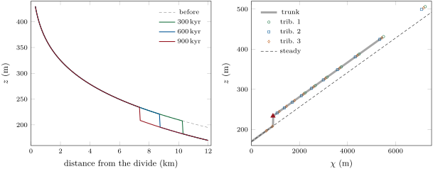
and any feature of the profile, a step included, travels upstream at the celerity $c = K A^m$ while keeping its height. A knickpoint starting at the outlet at $t = 0$ reaches the point $x$ at the time

$$t(x) = \int_0^x \frac{\mathrm{d}x'}{K A(x')^m} = \frac{\chi(x)}{K A_0^m},$$

with $\chi$ computed with $\theta = m$. All the knickpoints born in a network at the same time therefore lie at the same $\chi$, and on the same contour.

The celerity grows with drainage area: a knickpoint runs fast through the trunk and slows in the headwaters. The time it takes to cross the whole network to the channel heads is the response time of the landscape, of the order of a million years for typical uplift rates. When $n \ne 1$ the celerity also depends on the slope, and a step changes shape: for $n > 1$ its steep face outruns the reaches around it and stays sharp, for $n < 1$ it lags and spreads.

In the field — A waterfall that walks upstream

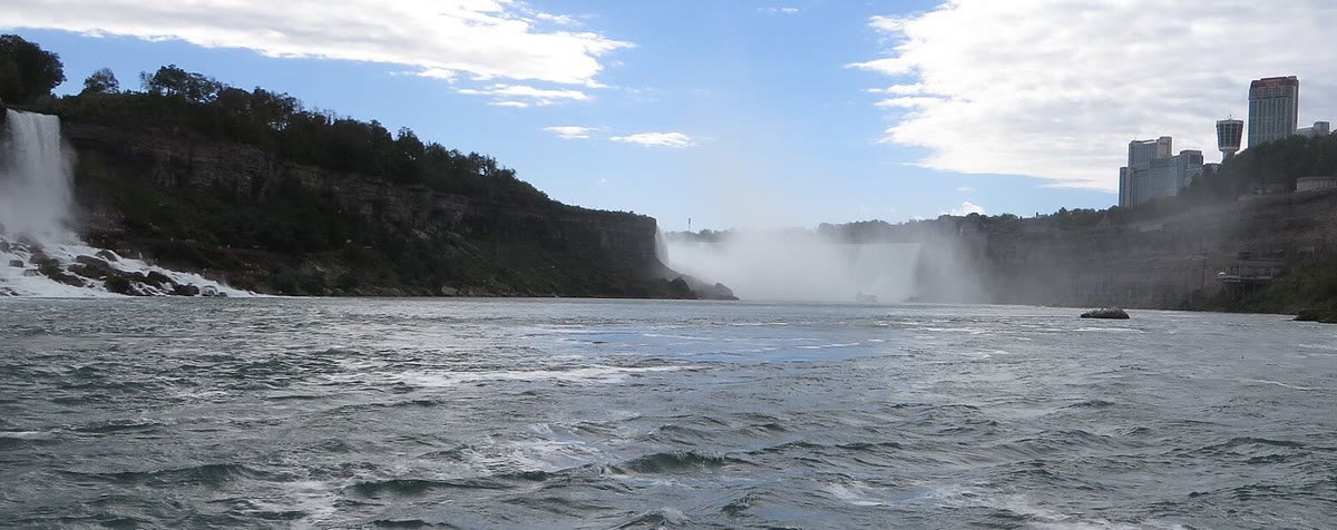
At Niagara the river drops into a gorge it has cut itself. About $12\,500$ years ago the Falls stood at the edge of the Niagara Escarpment; since then, as the water wore away the rocks of the escarpment and blocks broke from the crest, the crest has moved about $11\,\mathrm{km}$ upstream: about a metre a year on average, about a tenth of that today. Erosion is slower when the crest is a long horseshoe that spreads the water. The gorge is the path of the knickpoint.

18.4 Glacial erosion

A glacier sliding over its bed (basal sliding, Chapter 24) erodes it by abrasion, as debris held in the ice scours the rock, and by quarrying, as it pulls out blocks loosened by cracks. Both scale with the speed of sliding.

Definition 18.15 (Glacial erosion law)

A glacial erosion law gives the rate of erosion of a glacier’s bed as $E = K_G\,u_s^{\,l}$, where $u_s$ is the sliding speed, $K_G$ a coefficient and $l$ an exponent.

Landscape models usually take $l = 1$, with values between 1 and 2 in use. A compilation of 38 glaciers, whose erosion rates span five orders of magnitude, found erosion correlated with sliding speed, with $l = 0.65$ and $K_G = 10^{-4}$ for $E$ in metres a year: erosion is fastest under temperate glaciers fed by abundant snow, which slide fast. Since the ice is thickest and fastest along the axis of a valley, the floor is deepened more than the sides and the valley takes its U shape.

Definition 18.16 (Glacial buzzsaw)

The glacial buzzsaw is the limit set on the height of a mountain range by glaciers: where rock rises above the altitude at which glaciers form, they erode it as fast as it rises, whatever the uplift rate, so that peaks and mean elevation cluster near that altitude.

18.5 Tectonics and erosion

Definition 18.17 (Topographic steady state)

A landscape is in topographic steady state when its erosion rate equals the rock uplift rate everywhere, so that its elevations do not change though rock passes through it.

Rates measured over different spans of time test the state. Cosmogenic nuclides in river sand give the mean erosion rate of a basin over the time needed to remove a layer of the order of the attenuation length of their production, some $55\,\mathrm{cm}$ of rock; thermochronometers and their age–elevation relationships give the exhumation rate over millions of years. Where the two agree with each other and with the uplift rate, the landscape is likely in steady state; where the short-term rate is faster in the lower reaches than in the headwaters, a knickpoint is passing through. Removing rock also unloads the lithosphere, which rises in response.

Definition 18.18 (Erosional isostatic rebound)

Erosional isostatic rebound is the rise of the rock surface of a region in isostatic equilibrium in response to the mass removed by erosion.

Proposition 18.19 (Peaks rise as valleys deepen)

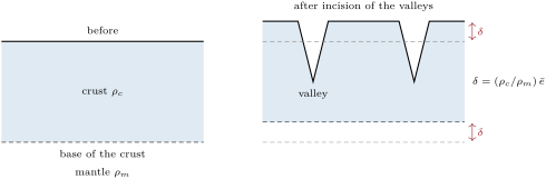
In Airy isostasy with crust of density $\rho_c$ over mantle of density $\rho_m$, removing a mean thickness $\bar e$ of crust from a region raises the whole region by $(\rho_c/\rho_m)\,\bar e$. If the erosion is confined to the valleys, the uneroded summits rise by that amount, while the mean surface falls by only $(1 - \rho_c/\rho_m)\,\bar e$.

The thickness-weighted density of the crust of the reference Earth model is $2.72\,\mathrm{g}/\mathrm{cm}^{3}$ and that of the mantle below its Moho $3.38\,\mathrm{g}/\mathrm{cm}^{3}$, a ratio of 0.80: of every hundred metres of rock eroded, the mean surface loses only twenty. Deep incision of an old plateau can thus raise its summits even as the plateau wears down.

18.6 Exercises

Exercise 18.1 ★

A shoreline scarp of offset $4\,\mathrm{m}$ ($a = 2\,\mathrm{m}$) stands on a far-field slope of 0.04, and its steepest gradient is now 0.30. Compute $\kappa t$, then the age of the scarp with $\kappa = 5 \times 10^{-3}\,\mathrm{m}^{2}/\mathrm{yr}$.

Solution

Solution of Exercise 18.1.

$a/\sqrt{\pi\kappa t} = 0.30 - 0.04 = 0.26$, so $\kappa t = (2/0.26)^2/\pi = 18.8\,\mathrm{m}^{2}$, and $t = 18.8/(5\times10^{-3}) = 3.8\,\mathrm{kyr}$, within a factor of two either way given the range of $\kappa$.

Exercise 18.2 ★

A lidar survey gives a hilltop curvature of $-0.012\,\mathrm{m}^{-1}$ on a ridge of diffusivity $4 \times 10^{-3}\,\mathrm{m}^{2}/\mathrm{yr}$. Compute its erosion rate in $\mathrm{mm}/\mathrm{yr}$, and the relief between its crest and channels $80\,\mathrm{m}$ away, assuming steady state.

Solution

Solution of Exercise 18.2.

$E = \kappa\,|\nabla^2 z| = 4\times10^{-3}\times0.012 = 4.8 \times 10^{-5}\,\mathrm{m}/\mathrm{yr}$, $0.048\,\mathrm{mm}/\mathrm{yr}$. Relief $E L^2/(2\kappa) = 0.012\times80^2/2 = 38.4\,\mathrm{m}$.

Exercise 18.3 ★

With $m = 0.5$, $n = 1$ and $K = 2 \times 10^{-6}\,\mathrm{yr}^{-1}$, compute the incision rate of a river draining $25\,\mathrm{km}^{2}$ on a gradient of 0.01. What are the units of $K$ for general $m$ and $n$?

Solution

Solution of Exercise 18.3.

$E = 2\times10^{-6}\times(25\times10^6)^{0.5}\times0.01 = 2\times10^{-6} \times5000\times0.01 = 1.0 \times 10^{-4}\,\mathrm{m}/\mathrm{yr}$, $0.1\,\mathrm{mm}/\mathrm{yr}$. Since $E$ is in $\mathrm{m}/\mathrm{yr}$, $A^m$ in $\mathrm{m}^{2m}$ and $S$ has no unit, $K$ is in $\mathrm{m}^{1-2m}\,\mathrm{yr}^{-1}$: $\mathrm{yr}^{-1}$ for $m = 0.5$.

Exercise 18.4 ★

Three rivers show knickpoints: (a) where a sandstone bed crosses a valley cut in shale; (b) where a river crosses an active normal fault from the footwall to the hanging wall; (c) in every river of a basin, all at about the same elevation, a few kilometres above a coast that rose in an earthquake. Which are fixed and which will migrate?

Solution

Solution of Exercise 18.4.

(a) Fixed: a hard bed steepens the river where it crops out, and the step stays with the bed. (b) Anchored at the fault: as long as the fault slips, the river is steepened where it crosses it. (c) Mobile: the uplift of the coast lowered the base level of every river at once; the knickpoints are migrating upstream and, as the kinematic-wave theorem predicts for $n = 1$, they lie on one contour.

Exercise 18.5 ★★

For $m = 1$ and $n = 2$, compute $\theta$ and the steady gradient where $A = 10\,\mathrm{km}^{2}$, with $U = 0.1\,\mathrm{mm}/\mathrm{yr}$ and $K = 10^{-9}$ in metres and years. By what factor does the steepness change if $U$ doubles? Compare with $n = 1$.

Solution

Solution of Exercise 18.5.

$\theta = m/n = 0.5$. $S = (U/K)^{1/2}A^{-1/2} = (10^{-4}/10^{-9})^{1/2} \times(10^7)^{-1/2} = 316\times3.16\times10^{-4} = 0.10$. Doubling $U$ multiplies $k_s = (U/K)^{1/n}$ by $\sqrt2 = 1.41$; for $n = 1$ by 2: the larger $n$, the less steepness responds to uplift.

Exercise 18.6 ★★

A river’s drainage area grows with the distance $d$ from its divide as $A = c\,d^{h}$. Show that, measured upstream from its outlet at $d = L$,

$$\chi(d) = \frac{A_0^{\theta}}{c^{\theta}}\,\frac{L^{p} - d^{p}}{p}, \qquad p = 1 - h\theta ,$$

and compute it for $c = 2$ (SI), $h = 1.8$, $\theta = 0.45$, $A_0 = 1\,\mathrm{km}^{2}$, $L = 20\,\mathrm{km}$ and $d = 5\,\mathrm{km}$.

Solution

Solution of Exercise 18.6.

With $x$ upstream from the outlet, $\mathrm{d}x = -\mathrm{d}d$, so $\chi(d) = \int_d^L (A_0/c\,d'^{h})^{\theta}\,\mathrm{d}d' = A_0^{\theta} c^{-\theta} \int_d^L d'^{-h\theta}\,\mathrm{d}d' = A_0^{\theta}c^{-\theta}(L^p - d^p)/p$. Here $p = 0.19$, $A_0^{\theta}c^{-\theta} = 10^{2.7}/2^{0.45}$, and $\chi = 2935\,\mathrm{m}$.

Exercise 18.7 ★★

With $n = 1$, $m = 0.5$ and $K = 2 \times 10^{-6}\,\mathrm{yr}^{-1}$, compute the celerity of a knickpoint where $A = 100\,\mathrm{km}^{2}$, in m/kyr, and the time it would take to travel $5\,\mathrm{km}$ at that speed. Why does it actually take longer?

Solution

Solution of Exercise 18.7.

$c = 2\times10^{-6}\times(10^8)^{0.5} = 0.02\,\mathrm{m}/\mathrm{yr}$, $20\,\mathrm{m}/\mathrm{kyr}$; $5\,\mathrm{km}$ at that speed takes $250\,\mathrm{kyr}$. The area, and with it the celerity, decreases upstream, so the knickpoint slows as it climbs.

Exercise 18.8 ★★

Valleys $600\,\mathrm{m}$ deep, occupying on average $40\,\%$ of the area of a plateau, are cut into it. With $\rho_c/\rho_m = 0.80$, compute the mean thickness eroded, the rise of the summits and the change of the mean elevation.

Solution

Solution of Exercise 18.8.

$\bar e = 0.40\times600 = 240\,\mathrm{m}$; the summits rise by $0.80\times240 = 192\,\mathrm{m}$; the mean elevation falls by $240 - 192 = 48\,\mathrm{m}$.

Exercise 18.9 ★★

A soil production function has $P_0 = 0.3\,\mathrm{mm}/\mathrm{yr}$ and $h_0 = 0.5\,\mathrm{m}$. Compute the steady soil thickness for erosion at $0.05\,\mathrm{mm}/\mathrm{yr}$ and at $0.2\,\mathrm{mm}/\mathrm{yr}$. What happens at $0.4\,\mathrm{mm}/\mathrm{yr}$?

Solution

Solution of Exercise 18.9.

$h = h_0\ln(P_0/E)$: $0.5\ln 6 = 0.90\,\mathrm{m}$ and $0.5\ln1.5 = 0.20\,\mathrm{m}$. At $0.4\,\mathrm{mm}/\mathrm{yr}$ erosion outpaces the fastest production, $P_0$: the soil is stripped and the slope becomes bare rock, its lowering limited by weathering.

Exercise 18.10 ★★★

A hill in steady state erodes at $E = 0.1\,\mathrm{mm}/\mathrm{yr}$ with $\kappa = 5 \times 10^{-3}\,\mathrm{m}^{2}/\mathrm{yr}$ and the nonlinear law of the critical gradient, taking $S_c = 1.2$ for the exercise. Show that the flux at a distance $x$ from the divide is $E x$, solve for the gradient, and compute it at 20, 50, 100 and $200\,\mathrm{m}$. Compare with linear diffusion and describe the shape of the hill.

Solution

Solution of Exercise 18.10.

At steady state $\mathrm{d}q/\mathrm{d}x = E$ and $q = 0$ at the divide, so $q = E x$. Then $\kappa S = E x\,(1 - S^2/S_c^2)$, a quadratic whose positive root is $S = [-\kappa + \sqrt{\kappa^2 + 4E^2x^2/S_c^2}\,]/(2Ex/S_c^2)$. At 20, 50, 100 and $200\,\mathrm{m}$: 0.36, 0.68, 0.89 and 1.03, against 0.4, 1.0, 2.0 and 4.0 for linear diffusion ($S = Ex/\kappa$). The hill has a rounded crest, then sides whose gradient tends to $S_c$: nearly planar slopes, much lower relief than the parabola.

Exercise 18.11 ★★★

Show that the response time of a river network to a change at its outlet, for $n = 1$, is $\chi_h/(K A_0^m)$, where $\chi_h$ is the largest value of $\chi$ at a channel head. Compute it for the upland river of the figures ($A_0 = 1\,\mathrm{km}^{2}$, $m = 0.5$, $K = 10^{-6}\,\mathrm{yr}^{-1}$), first for its trunk alone, whose head is at $\chi = 5464\,\mathrm{m}$, then for the network, whose highest head, on tributary 1, is at $\chi = 7237\,\mathrm{m}$.

Solution

Solution of Exercise 18.11.

By the kinematic-wave theorem the change reaches a point of coordinate $\chi$ after $\chi/(KA_0^m)$; the network has fully responded when it has reached the last channel head, of largest $\chi$. $K A_0^m = 10^{-6}\times 1000 = 10^{-3}\,\mathrm{m}/\mathrm{yr}$: the trunk responds in $5.46\,\mathrm{Myr}$, the network in $7.24\,\mathrm{Myr}$, the order of a million years expected.

Exercise 18.12 ★★★

In a network with $n = 1$ and uniform $U$, one tributary flows on rock twice as erodible as the rest ($2K$) above its junction, at $\chi_j$. Show that its steady-state line in the $(\chi, z)$ plane has half the slope of the trunk’s above $\chi_j$, and that a knickpoint born at the outlet reaches, at the time when the trunk’s knickpoint is at $\chi_k > \chi_j$, the point of $\chi = \chi_j + 2(\chi_k - \chi_j)$ of that tributary.

Solution

Solution of Exercise 18.12.

Above the junction the tributary’s steady gradient is $S = (U/2K)A^{-\theta}$, so $\mathrm{d}z/\mathrm{d}\chi = (U/2K)A_0^{-\theta}$, half the trunk’s. The knickpoint reaches the junction when the trunk’s is at $\chi_j$; after a further time $\Delta t$ the trunk’s has moved to $\chi_k$ with $\chi_k - \chi_j = K A_0^m\,\Delta t$, while the tributary’s, with celerity $2KA^m$, has moved to $\chi$ with $\chi - \chi_j = 2KA_0^m\,\Delta t = 2(\chi_k - \chi_j)$.

18.7 Problem: The Waterfall of the Varden River

Problem 18.1

Weekend problem — the profile, steepness and erodibility of an invented upland river, and the age of its waterfall

West of the Varden Hills, the river drains an upland of schist before it enters the map at its west edge, at an elevation of $170\,\mathrm{m}$. Upstream of that point, its outlet, the trunk is $12\,\mathrm{km}$ long from its divide, with a drainage area $A = 4.5\,d^{1.7}$ ($\mathrm{m}^{2}$, $d$ in metres from the divide) and a channel head at $d = 300\,\mathrm{m}$. Take as the rate of rock uplift the denudation rate of the Varden river’s basin found from its loads in the Year 1 volume, $43\,\mathrm{m}/\mathrm{Myr}$. Take $n = 1$ and the reference area $A_0 = 1\,\mathrm{km}^{2}$. A waterfall $25\,\mathrm{m}$ high stands on the trunk $4.60\,\mathrm{km}$ upstream of the outlet. All values are invented.

Part I — The profile.

1. Compute the drainage area at the outlet and at the channel head.

2. Gradients measured over reaches of $200\,\mathrm{m}$, away from the waterfall:

   $A$ ($\mathrm{km}^{2}$)	0.388	0.587	0.888	1.345	2.036	3.082
   $S$	0.06641	0.05026	0.04888	0.03322	0.03688	0.02688
   $A$ ($\mathrm{km}^{2}$)	4.665	7.061	10.69	16.18	24.49	37.08
   $S$	0.01921	0.01713	0.01545	0.01419	0.007922	0.007855

   Estimate the concavity index from the first and last points.

3. The least-squares slope of $\log S$ against $\log A$ is $-0.466$. Is it consistent with $\theta = 0.5$?
4. With $\theta_{\mathrm{ref}} = 0.5$, compute $k_{sn} = S A^{0.5}$ ($A$ in $\mathrm{m}^{2}$) for the first and the last point, and say what the geometric mean of the twelve values, $45.1\,\mathrm{m}$, represents.
5. Why do gradients scatter so much more than elevations?
6. Using the formula of the chi exercise, compute $\chi$ at $d = 9.00\,\mathrm{km}$, a point below the waterfall.

Part II — Steepness and erodibility.

7. The river is at $193.4\,\mathrm{m}$ at $d = 9.00\,\mathrm{km}$. Compute the slope of the chi plot below the waterfall and the steepness $k_{sn}$.
8. Which estimate of $k_{sn}$, this one or the slope-area one, would you trust, and why?
9. Assuming steady state below the waterfall, compute $K$ from the uplift rate.
10. Check that the incision rate at the outlet, whose gradient is 0.00691, equals the uplift rate.
11. Compute the celerity of a knickpoint at the outlet and at the waterfall, in m/kyr.
12. Compute the elevation of the channel head on the steady profile, and the relief of the trunk.

Part III — The waterfall.

13. Why, with $n = 1$, has the waterfall kept the height of the fall of base level?
14. Compute $\chi$ at the waterfall.
15. Compute the time the knickpoint took from the outlet to its present place.
16. Where will it be $300\,\mathrm{kyr}$ from now?
17. Tributary 3 joins the trunk $2.5\,\mathrm{km}$ upstream of the outlet; it is $5\,\mathrm{km}$ long, with $A = 1.5\,s^{1.7}$ ($s$ from its own divide). Where should its waterfall be?
18. Tributaries 1 and 2 join the trunk 8 and $5\,\mathrm{km}$ upstream of the outlet. Explain why they have no waterfall.

Part IV — The hillslopes and the age.

19. A lidar survey above the waterfall gives a hilltop curvature of $-0.0086\,\mathrm{m}^{-1}$. With $\kappa = 5 \times 10^{-3}\,\mathrm{m}^{2}/\mathrm{yr}$, compute the erosion rate and compare it with the uplift rate.
20. The hillslopes are about $150\,\mathrm{m}$ long. Compare their response time $L^2/\kappa$ with the age found in Part III.
21. Describe the hillslopes below the waterfall today, and how they will change.
22. The uplift rate is known to $20\,\%$. Give the range of the age.
23. How would the waterfall have evolved if $n$ were 2?
24. Give the age of the fall of base level.

Solution

Solution of Problem 18.1.

1. $4.5\times12000^{1.7} = 3.87 \times 10^{7}\,\mathrm{m}^{2}$, $38.7\,\mathrm{km}^{2}$; $4.5\times300^{1.7} = 7.3 \times 10^{4}\,\mathrm{m}^{2}$, $0.073\,\mathrm{km}^{2}$.

2. $\theta \approx -\log(0.007855/0.06641)/\log(37.08/0.388) = 0.928/1.980 = 0.47$.

3. Yes: with a scatter of about $10\,\%$ on twelve points, $0.466$ does not differ significantly from 0.5.

4. $0.06641\times\sqrt{388\,000} = 41.4\,\mathrm{m}$; $0.007855\times\sqrt{3.708\times10^7} = 47.8\,\mathrm{m}$. The geometric mean, $45.1\,\mathrm{m}$, estimates $k_s$ for $\theta = 0.5$.

5. A gradient is the difference of two elevations, each uncertain by decimetres to metres, divided by a short distance; on gentle reaches the error is a large part of the difference. $\chi$ integrates instead of differentiating.

6. $p = 1 - 1.7\times0.5 = 0.15$; $\chi = (1000/\sqrt{4.5})\, (12000^{0.15} - 9000^{0.15})/0.15 = 543.1\,\mathrm{m}$.

7. $(193.4 - 170)/543.1 = 0.0431$; $k_{sn} = 0.0431\times A_0^{0.5} = 43.1\,\mathrm{m}$.

8. The chi estimate: it rests on elevations over $3\,\mathrm{km}$ of river, not on twelve noisy gradients.

9. $K = U/k_{sn} = 4.3\times10^{-5}/43.1 = 1.00 \times 10^{-6}\,\mathrm{yr}^{-1}$.

10. $10^{-6}\times\sqrt{3.87\times10^7}\times0.00691 = 4.30 \times 10^{-5}\,\mathrm{m}/\mathrm{yr}$, $43\,\mathrm{m}/\mathrm{Myr}$: the outlet keeps pace with the uplift.

11. At the outlet $10^{-6}\times6222 = 6.2\,\mathrm{m}/\mathrm{kyr}$; at the waterfall, $d = 7.40\,\mathrm{km}$, $A = 1.70 \times 10^{7}\,\mathrm{m}^{2}$ and $4.1\,\mathrm{m}/\mathrm{kyr}$.

12. $170 + 43\times(4.5)^{-0.5}(12000^{0.15} - 300^{0.15})/0.15 = 405\,\mathrm{m}$: a relief of $235\,\mathrm{m}$.

13. For $n = 1$ the equation is a kinematic wave: points on both sides of the step rise by $U$ per unit time, so the step keeps its height, the $25\,\mathrm{m}$ of the fall.

14. $\chi = (1000/\sqrt{4.5})(12000^{0.15} - 7400^{0.15})/0.15 = 899.4\,\mathrm{m}$.

15. $t = \chi/(KA_0^{0.5}) = 899.4/10^{-3} = 899\,\mathrm{kyr}$.

16. At $\chi = 899.4 + 300 = 1199\,\mathrm{m}$: $d^{0.15} = 12000^{0.15} - 1199\times0.15\times\sqrt{4.5}/1000$, $d = 6.25\,\mathrm{km}$, $5.75\,\mathrm{km}$ upstream of the outlet.

17. At the junction ($d = 9.5\,\mathrm{km}$) $\chi = 442.8\,\mathrm{m}$; the waterfall lies where the tributary’s $\chi$ reaches $899.4\,\mathrm{m}$: $s^{0.15} = 5000^{0.15} - (899.4 - 442.8)\times0.15\times\sqrt{1.5}/1000$, $s = 4.27\,\mathrm{km}$, $0.73\,\mathrm{km}$ above the junction.

18. Their junctions are at $\chi = 1954$ and $999\,\mathrm{m}$, beyond $899\,\mathrm{m}$: the knickpoint has not yet passed them, so the trunk there is still at its old level.

19. $E = 5\times10^{-3}\times0.0086 = 4.3 \times 10^{-5}\,\mathrm{m}/\mathrm{yr}$, $43\,\mathrm{m}/\mathrm{Myr}$: the hills above the waterfall erode at the uplift rate, in steady state.

20. $150^2/(5\times10^{-3}) = 4.5\,\mathrm{Myr}$, five times the age of the waterfall.

21. Their foot was lowered $25\,\mathrm{m}$ with the channel: their lower parts are oversteepened, perhaps sliding, while their crests still erode at the old rate. A wave of steepening climbs each slope; after a few million years they return to the same parabola, $25\,\mathrm{m}$ lower.

22. $t = \chi k_{sn}/(U A_0^{0.5})$ varies as $1/U$: from $899/1.2 = 749$ to $899/0.8 = 1124\,\mathrm{kyr}$.

23. With $n = 2$ the celerity grows with the gradient: the steep face would travel faster than the reaches around it and stay sharp, but its speed and the age read from it would differ.

24. The base level of the Varden river fell $900\,\mathrm{kyr}$ ago ($899\,\mathrm{kyr}$ by the calculation).