2Exploration Seismology

A survey vessel steams slowly along a straight line at sea, towing an array of air guns a few metres below the surface and, behind it, cables several kilometres long studded with hydrophones. In one survey described to the regulator, the array held $5240$ cubic inches of compressed air, fired every $8\,\mathrm{s}$ from $12\,\mathrm{m}$ below the surface, and the narrow-azimuth streamers behind such vessels record offsets of 8 to $10\,\mathrm{km}$.

Each shot sends a pulse of sound into the sea floor, and every rock interface below returns a faint echo. Weeks of processing later, a geologist scrolls through a cross-section in which buried river channels, tilted fault blocks and the onlapping fill of an old basin appear as if the ground had been cut open. The Earth-scale seismology of the previous chapter used the waves of earthquakes; exploration seismology makes its own, with sources whose time and place are known exactly, and records them on thousands of channels. This chapter follows the echoes from the shot to the section: refraction surveys, the reflection of a wavelet by a layered column, the common-midpoint method that turns repeated echoes into velocities and a clean image, migration, which puts the reflectors back where they belong, and the reading of the section as stratigraphy.

You already know

At a boundary between two media of acoustic impedances $Z_1 = \rho_1v_1$ and $Z_2 = \rho_2v_2$, a plane wave at normal incidence is reflected with the amplitude coefficient $R = (Z_2 - Z_1)/(Z_2 + Z_1)$ (the physics books’ Year 2 volume, on waves at interfaces). The head wave, the intercept time and the crossover distance of a refraction profile over flat layers were met in the Year 1 volume, in its chapter on the layered Earth; borehole logs in Book 2 (grade 11). The convolution $(f*g)(t) = \int f(\tau)g(t - \tau)\,\mathrm d\tau$ and the Fourier transform are the mathematics books’. The ray parameter and the linear inverse problem are those of Chapter 1.

2.1 Refraction surveys

Definition 2.1 (Seismic refraction and reflection surveys)

A seismic refraction survey records, along a line of receivers, the first arrivals from a controlled source, and uses the head waves that travel along the top of faster layers to find their speeds and depths. A seismic reflection survey records the whole wave train, at offsets mostly smaller than the depths of interest, and uses the waves reflected at near-normal incidence by the interfaces to image the layering.

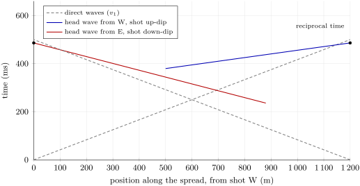
Over flat layers a head wave arrives at $t = x/v_2 + t_i$, a straight line whose slope gives the speed $v_2$ of the refractor and whose intercept $t_i$ gives its depth. A dipping refractor tilts the line: the head wave shot down-dip arrives later and later, as the refractor goes deeper, and seems slow; shot up-dip it seems fast. Shooting both ways along the same line, a reversed profile, separates the speed from the dip.

Theorem 2.2 (Refraction on a dipping interface)

A layer of speed $v_1$ overlies a plane refractor of speed $v_2 > v_1$ dipping at the angle $\theta$ along the profile; $i_c = \arcsin(v_1/v_2)$, and $h$ is the perpendicular depth of the refractor under the shot. Beyond the critical distance, the head wave arrives at

$$\begin{align*} t &= \frac{x\sin(i_c + \theta)}{v_1} + \frac{2h\cos i_c}{v_1} &&\text{shooting down-dip},\\ t &= \frac{x\sin(i_c - \theta)}{v_1} + \frac{2h\cos i_c}{v_1} &&\text{shooting up-dip}. \end{align*}$$

The apparent speeds $v_d = v_1/\sin(i_c + \theta)$ and $v_u = v_1/\sin(i_c - \theta)$ of a reversed profile give

$$i_c = \tfrac12\left[\arcsin\frac{v_1}{v_d} + \arcsin\frac{v_1}{v_u}\right],\qquad \theta = \tfrac12\left[\arcsin\frac{v_1}{v_d} - \arcsin\frac{v_1}{v_u}\right], \qquad v_2 = \frac{v_1}{\sin i_c} .$$

The two branches of a reversed profile must give the same time between the two shot points, whichever end fired: the reciprocal time, a check on the picking. Two situations defeat the method. A layer slower than the one above it (a velocity inversion) refracts no head wave and is invisible: its rocks are counted in the layer above, and every depth below is overestimated. A layer faster than the one above but too thin may never give a first arrival, because the head wave of the deeper, faster layer overtakes it: a hidden layer. A reflection survey sees both.

2.2 Reflection at normal incidence

Definition 2.3 (Seismic wavelet, Ricker wavelet)

A seismic wavelet is the short pulse, a few tens of milliseconds long, that a source and the recording system send through the ground; each reflector returns a scaled copy of it. The Ricker wavelet of peak frequency $f$ is the zero-phase pulse

$$w(t) = \left(1 - 2\pi^2f^2t^2\right)e^{-\pi^2f^2t^2},$$

the second derivative of a Gaussian, up to sign and scale: a central peak and two side lobes, with zero mean and an amplitude spectrum peaking at $f$.

Definition 2.4 (Reflectivity series)

The reflectivity series of a layered column is the sequence of normal-incidence reflection coefficients $r_k$ of its interfaces, placed at their two-way vertical times $\tau_k = \sum_{i \le k} 2h_i/v_i$: $r(t) = \sum_k r_k\,\delta(t - \tau_k)$.

Proposition 2.5 (The convolutional model)

If only primary reflections are kept (no multiples), at normal incidence, with no transmission loss, attenuation or spreading, and the wavelet $w$ does not change with depth, the recorded trace is the convolution of the wavelet with the reflectivity series:

$$s(t) = \sum_k r_k\,w(t - \tau_k) = (w*r)(t) .$$

The trace computed in this way from a borehole log of speed and density is the synthetic seismogram of the log.

The synthetic seismogram is how a borehole is tied to a seismic section: a reflection on the section is matched to the interface of the log that makes it. The Varden column beneath the syncline axis of the problem (the seismic model of this chapter, with speeds and densities chosen within published ranges for each rock)

gives the figure below. The chalk–shale interface reflects only $2.8\,\%$ of the amplitude, because chalk and shale happen to have almost the same impedance; the top of the limestone reflects $38\,\%$, the base of the limestone sends back a reversed pulse, and the basement a strong positive one.

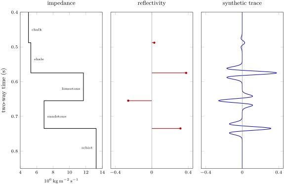
How thin a layer can the reflections still resolve? Its top and its base each return a wavelet; when they overlap, they interfere.

Definition 2.6 (Tuning thickness)

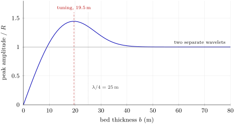
The tuning thickness of a bed is the thickness at which the reflections from its top and base, of opposite signs, interfere most constructively, so that the composite amplitude is greatest. Thinner beds are not resolved: their top and base can no longer be picked separately, and the amplitude decreases in proportion to the thickness.

Proposition 2.7 (Quarter-wavelength rule)

For a wavelet of dominant period $T$ in a bed of speed $v$, with reflection coefficients $+R$ at its top and $-R$ at its base, the composite reflection is strongest when the bed thickness is $b = \lambda/4$, where $\lambda = vT$; for $b \ll \lambda/4$ its amplitude is proportional to $b$.

A Ricker wavelet is not a harmonic, and its tuning thickness, read off the wedge model of the figure below, is a little smaller than a quarter of the wavelength at the peak frequency: $19.5\,\mathrm{m}$ at $30\,\mathrm{Hz}$ in rock of $3000\,\mathrm{m}\,\mathrm{s}^{-1}$, for $\lambda/4 = 25\,\mathrm{m}$. Seismic data rarely contain much energy above a few tens of hertz from depths of kilometres, because the rocks absorb the high frequencies; beds less than about $20\,\mathrm{m}$ thick are seen as a single reflection.

Laterally, the resolution is set by the width of the reflector that sends energy back in phase.

Definition 2.8 (Fresnel zone)

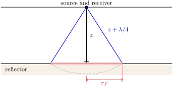
The (first) Fresnel zone of a reflector, for a coincident source and receiver at height $z$ above it, is the disc of reflector around the normal-incidence point from which the two-way path is longer than the normal path by less than half a wavelength: its reflections arrive in phase and build the recorded reflection together.

Proposition 2.9 (Radius of the Fresnel zone)

The first Fresnel zone has the radius $r_F = \sqrt{\lambda z/2 + \lambda^2/16} \approx \sqrt{\lambda z/2}$ for $\lambda \ll z$.

At $1\,\mathrm{km}$ depth, with $\lambda = 100\,\mathrm{m}$, the Fresnel zone is $225\,\mathrm{m}$ in radius: features narrower than that are smeared, unless migration (below) collapses the zone.

2.3 Common-midpoint acquisition and processing

A single echo is too faint to see in the noise. Reflection surveys therefore record each subsurface point many times, with different source–receiver pairs, and add the records.

Definition 2.10 (Common midpoint, fold)

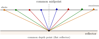
For a source at $x_s$ and a receiver at $x_r$ on a line, the midpoint is $(x_s + x_r)/2$ and the offset $x = |x_r - x_s|$. A common midpoint (CMP) gather is the set of traces, from all the shots, that share the same midpoint; over flat layers they all reflect from the same subsurface point. The fold (of seismic coverage) is the number of traces in a gather. With $N$ channels at the receiver interval $\Delta g$ and a shot every $\Delta s$ along the line, the fold is $N\Delta g/(2\Delta s)$.

Theorem 2.11 (Normal moveout)

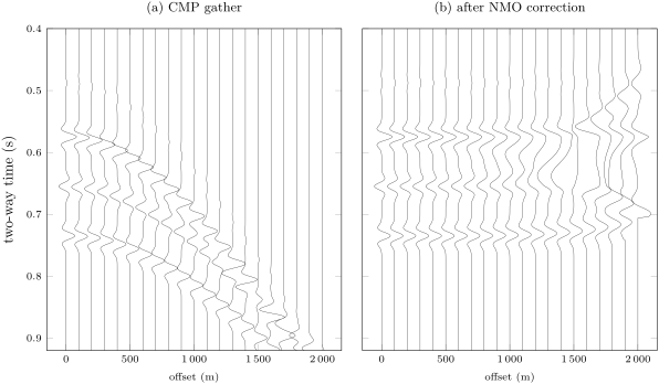
In a layer of speed $v$ over a flat reflector at the two-way vertical time $t_0$, the reflection recorded at offset $x$ arrives at

$$t(x)^2 = t_0^2 + \frac{x^2}{v^2},$$

a hyperbola in the $(x, t)$ plane. The delay $\Delta t = t(x) - t_0$ is the normal moveout; for $x \ll vt_0$, $\Delta t \approx x^2/(2v^2t_0)$.

Over several layers the reflection time is no longer exactly hyperbolic, but it is nearly so at small offsets, with a speed that is a weighted mean of the layers’.

Definition 2.12 (Stacking, root-mean-square and interval velocities)

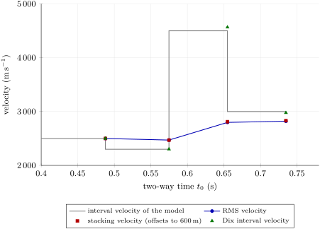
The interval velocity $v_i$ of a layer is its own speed; with $\Delta t_i = 2h_i/v_i$ the two-way time across it, the root-mean-square velocity down to the base of layer $n$ is

$$V_{\text{rms},n} = \left(\frac{\sum_{i\le n}v_i^2\,\Delta t_i}{\sum_{i\le n}\Delta t_i}\right)^{1/2}.$$

The stacking velocity of a reflection is the speed $V$ of the hyperbola $t^2 = t_0^2 + x^2/V^2$ that best fits its times in a CMP gather.

Proposition 2.13 (Stacking velocity at small offsets)

Over flat layers, $t(x)^2 = t_0^2 + x^2/V_{\text{rms}}^2 + O(x^4)$: at small offsets, the stacking velocity is the RMS velocity.

Theorem 2.14 (Dix equation)

If $V_{n-1}$ and $V_n$ are the RMS velocities to the top and the base of layer $n$, at the two-way times $t_{n-1}$ and $t_n$, the interval velocity of the layer is given by the Dix equation

$$v_n^2 = \frac{V_n^2t_n - V_{n-1}^2t_{n-1}}{t_n - t_{n-1}} ,$$

and its thickness is $h_n = v_n(t_n - t_{n-1})/2$.

Velocity analysis scans each gather for the hyperbola that best fits the energy: for each trial $t_0$ and $V$, the traces are summed along the curve, and a coherence measure (the semblance) is mapped; the analyst picks its maxima, reflector by reflector, to build a velocity function. The NMO correction then shifts every sample of every trace from $t(x)$ to $t_0$, flattening the reflections, and the traces of each gather are added.

Definition 2.15 (Stacking (seismic))

Stacking (seismic) is the summation, after the normal-moveout correction, of the traces of a CMP gather into a single trace placed at the midpoint. The stacked traces, side by side along the line, form the stacked section, an image of the reflectors in two-way time.

Proposition 2.16 (Gain of a stack)

If the $N$ traces of a gather carry the same reflection signal and independent noise of equal standard deviation $\sigma$, their mean carries the same signal and noise of standard deviation $\sigma/\sqrt N$: stacking raises the signal-to-noise ratio by $\sqrt N$.

2.4 Migration

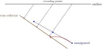
A stacked section shows each reflection under the midpoint where it was recorded, at the time it took to come back. For a flat reflector that is where it is. For a dipping one it is not: the echo recorded at a surface point comes from the point of the reflector nearest to it, which lies up-dip, not vertically below. Points such as fault cut-offs, which scatter energy in all directions, appear as hyperbolae.

Definition 2.17 (Seismic migration)

Seismic migration is the processing step that moves the reflections of a seismic section to the positions of the reflectors that produced them: it restores the true dips and positions of dipping reflectors and collapses the diffraction hyperbolae of point scatterers onto their apices. Done with a velocity model in time, it gives a time-migrated section; with a model in depth, a depth image.

Theorem 2.18 (Dip on a zero-offset section)

In a medium of speed $v$, a plane reflector of dip $\theta$ in the plane of the section appears on the zero-offset section, plotted as the depth $vt/2$ vertically below each recording point, as a line of apparent dip $\theta_a$ with

$$\tan\theta_a = \sin\theta .$$

The reflection recorded at the point $x$ comes from the reflector point a distance $(vt/2)\sin\theta$ up-dip of the point vertically below $x$.

Since $\tan\theta_a = \sin\theta < \tan\theta$, an unmigrated section always shows dips gentler than the true ones, and it cannot show dips steeper than $45{}^{\circ}$ at all. A point scatterer at depth $z$ below the point $x_0$ returns at $x$ the zero-offset time $t(x) = (2/v)\sqrt{z^2 + (x - x_0)^2}$: a hyperbola with its apex over the point, the diffraction. Migration in its simplest form, the diffraction stack, sums each section along the diffraction hyperbola of every possible scatterer and puts the sum at the apex: reflectors, which are continuous lines of scatterers, emerge in their true places, and the diffractions collapse.

2.5 Seismic stratigraphy

A migrated section is a picture of the layering, and it can be read as stratigraphy: the reflections follow the bedding surfaces, which are time lines, so their geometry records how the basin filled.

Definition 2.19 (Seismic stratigraphy, seismic facies)

Seismic stratigraphy is the interpretation of the stratigraphy and depositional history of a basin from the geometry of its seismic reflections. A seismic facies is a three-dimensional unit of reflections whose character (continuity, amplitude, frequency, internal geometry: parallel, divergent, sigmoid, chaotic, mounded) differs from that of its neighbours and is interpreted as a depositional environment.

Definition 2.20 (Reflection terminations)

A reflection termination is the end of a reflection against another. Onlap: an initially horizontal reflection ends against a surface that rises more steeply, the younger beds lapping onto an older slope. Downlap: an inclined reflection ends down-dip against a gentler surface, as the toes of prograding beds rest on the floor of a basin. Toplap: inclined reflections end up-dip against an overlying surface, with little erosion, as the tops of prograding beds meet the level of the sea. Erosional truncation: reflections end up-dip against an overlying surface that cuts them, an unconformity.

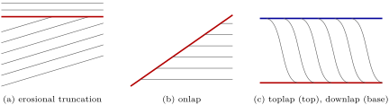
The terminations mark the surfaces that bound sequences of genetically related beds; mapping them across a basin, and relating them to the rise and fall of relative sea level, is sequence stratigraphy, the subject of Chapter 16. A seismic section of a passive margin typically shows wedges of seaward-prograding reflections downlapping onto the deep floor, capped by toplap, and buried landward under onlapping beds laid down when the sea rose again.

In the field — A marine streamer survey and a land crew

On a marine survey the vessel never stops: it sails line after line at a few knots, the air-gun arrays firing at fixed intervals, the streamers held at a constant depth by small steerable wings and located by acoustic and satellite positioning. Observers on the bridge watch the sea around the array, and the survey works under rules that set out the measures to protect marine mammals, the watch kept and what is reported.

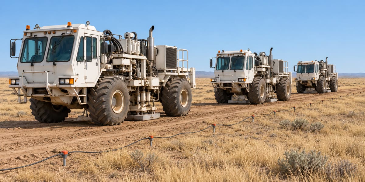
On land the crew lays out cables or wireless recording units along the lines; vibrator trucks advance in convoy from one source point to the next, and a recording truck checks every channel before each sweep. Back in the processing centre the records are sorted into common-midpoint gathers, the velocities picked, the data stacked and migrated, and the section handed to the interpreters.

2.6 Exercises

Exercise 2.1 ★

Chalk ($v = 2500\,\mathrm{m}\,\mathrm{s}^{-1}$, $\rho = 2.00\,\mathrm{g}\,\mathrm{cm}^{-3}$) lies on shale ($2300\,\mathrm{m}\,\mathrm{s}^{-1}$, $2.30\,\mathrm{g}\,\mathrm{cm}^{-3}$), which lies on limestone ($4500\,\mathrm{m}\,\mathrm{s}^{-1}$, $2.60\,\mathrm{g}\,\mathrm{cm}^{-3}$). Compute the three impedances and the reflection coefficients of the two interfaces. What fraction of the incident energy does the top of the limestone reflect?

Solution

Solution of Exercise 2.1.

$Z = \rho v$: chalk $2000\times2500 = 5.00 \times 10^{6}\,\mathrm{kg}\,\mathrm{m}^{-2}\,\mathrm{s}^{-1}$, shale $2300\times2300 = 5.29 \times 10^{6}\,\mathrm{kg}\,\mathrm{m}^{-2}\,\mathrm{s}^{-1}$, limestone $2600\times4500 = 11.70 \times 10^{6}\,\mathrm{kg}\,\mathrm{m}^{-2}\,\mathrm{s}^{-1}$. Chalk–shale: $R = (5.29 - 5.00)/(5.29 + 5.00) = 0.29/10.29 = 0.0282$; shale–limestone: $R = (11.70 - 5.29)/(11.70 + 5.29) = 6.41/16.99 = 0.377$. The reflected energy is $R^2 = 0.142$: the top of the limestone sends back $14.2\,\%$ of the incident energy, the chalk–shale interface less than $0.1\,\%$.

Exercise 2.2 ★

A flat reflector lies $800\,\mathrm{m}$ below a layer of $2000\,\mathrm{m}\,\mathrm{s}^{-1}$. Compute $t_0$, the reflection time at an offset of $1000\,\mathrm{m}$, and the normal moveout there. Compare with the approximation $x^2/(2v^2t_0)$.

Solution

Solution of Exercise 2.2.

$t_0 = 2\times800/2000 = 0.800\,\mathrm{s}$; $t = \sqrt{0.800^2 + (1000/2000)^2} = \sqrt{0.89} = 0.9434\,\mathrm{s}$; the moveout is $0.1434\,\mathrm{s}$. The approximation gives $1000^2/(2\times2000^2\times0.800) = 0.1563\,\mathrm{s}$, too large by $9\,\%$: at an offset larger than the depth, $x \ll vt_0$ no longer holds.

Exercise 2.3 ★

A streamer has 240 channels $12.5\,\mathrm{m}$ apart, and the vessel fires every $25\,\mathrm{m}$. Compute the CMP interval and the fold. What shot interval would give a fold of 120?

Solution

Solution of Exercise 2.3.

Midpoints move by half the receiver interval: the CMP interval is $12.5/2 = 6.25\,\mathrm{m}$. The fold is $240\times12.5/(2\times25) = 60$. A fold of 120 needs a shot every $240\times12.5/(2\times120) = 12.5\,\mathrm{m}$.

Exercise 2.4 ★

With a dominant frequency of $30\,\mathrm{Hz}$, compute the wavelength and the quarter wavelength in sandstone of $3000\,\mathrm{m}\,\mathrm{s}^{-1}$ and in limestone of $4500\,\mathrm{m}\,\mathrm{s}^{-1}$. Compute the radius of the first Fresnel zone of a reflector $1000\,\mathrm{m}$ deep under rocks of mean speed $2800\,\mathrm{m}\,\mathrm{s}^{-1}$.

Solution

Solution of Exercise 2.4.

$\lambda = v/f$: $100\,\mathrm{m}$ in the sandstone, $\lambda/4 = 25\,\mathrm{m}$; $150\,\mathrm{m}$ in the limestone, $\lambda/4 = 37.5\,\mathrm{m}$. With $\lambda = 2800/30 = 93.3\,\mathrm{m}$ and $z = 1000\,\mathrm{m}$, $r_F \approx \sqrt{\lambda z/2} = \sqrt{46\,667} = 216\,\mathrm{m}$ ($217\,\mathrm{m}$ with the term $\lambda^2/16$).

Exercise 2.5 ★★

Two reflections have $t_0 = 0.500\,\mathrm{s}$ with an RMS velocity of $2400\,\mathrm{m}\,\mathrm{s}^{-1}$, and $t_0 = 0.700\,\mathrm{s}$ with $2800\,\mathrm{m}\,\mathrm{s}^{-1}$. Compute the interval velocity and the thickness of the layer between them.

Solution

Solution of Exercise 2.5.

Dix: $v^2 = (2800^2\times0.700 - 2400^2\times0.500)/0.200 = (5\,488\,000 - 2\,880\,000)/0.200 = 1.304 \times 10^{7}\,\mathrm{m}^{2}\,\mathrm{s}^{-2}$, so $v = 3611\,\mathrm{m}\,\mathrm{s}^{-1}$. The layer is crossed in $0.100\,\mathrm{s}$ one way: $h = 3611\times0.100 = 361\,\mathrm{m}$.

Exercise 2.6 ★★

A plane reflector dips at $\varphi$ in the plane of a CMP line, in a layer of speed $v$. (a) Show that $t(x)^2 = t_0^2 + x^2\cos^2\varphi/v^2$, where $t_0$ is the zero-offset time at the midpoint. (Hint: use the image of the midpoint in the reflector.) (b) Deduce the stacking velocity, and compute it for $v = 2000\,\mathrm{m}\,\mathrm{s}^{-1}$ and $\varphi = 12{}^{\circ}$.

Solution

Solution of Exercise 2.6.

(a) Let $d$ be the distance from the midpoint M to the reflector, so that $t_0 = 2d/v$. The reflected ray from the source S to the receiver G is as long as the straight line from the image S$'$ of S in the reflector to G. Put M at the origin, the line along the dip; S$'$ lies at the distance $2d_S$ from S along the normal, with $d_S = d - (x/2)\sin\varphi$. The square of S$'$G is $x^2 + 4d_S^2 + 4d_Sx\sin\varphi = x^2 + 4d^2 - x^2\sin^2\varphi$, all the terms in $dx$ cancelling, so $v^2t^2 = 4d^2 + x^2\cos^2\varphi$ and $t^2 = t_0^2 + x^2\cos^2\varphi/v^2$. (b) The gather follows a hyperbola of speed $V = v/\cos\varphi = 2000/\cos12{}^{\circ} = 2045\,\mathrm{m}\,\mathrm{s}^{-1}$: a dip makes the stacking velocity too high, here by $2.2\,\%$.

Exercise 2.7 ★★

A gather of fold 60 has independent noise of equal variance on every trace. By what factor does stacking raise the signal-to-noise ratio? By what factor must the fold be increased to double it again?

Solution

Solution of Exercise 2.7.

By $\sqrt{60} = 7.75$. Doubling the signal-to-noise ratio needs four times as many traces: a fold of 240.

Exercise 2.8 ★★

On a zero-offset time section, in rock of $3000\,\mathrm{m}\,\mathrm{s}^{-1}$, a reflection rises by $0.40\,\mathrm{s}$ of two-way time per kilometre along the line. Convert this slope into an apparent dip, and compute the true dip of the reflector.

Solution

Solution of Exercise 2.8.

The plotted depth $vt/2$ changes by $1.5\,\mathrm{km}\,\mathrm{s}^{-1}\times0.40\,\mathrm{s} = 0.60\,\mathrm{km}$ per kilometre: $\tan\theta_a = 0.60$, $\theta_a = 31.0{}^{\circ}$. By the zero-offset theorem $\sin\theta = 0.60$: $\theta = 36.9{}^{\circ}$.

Exercise 2.9 ★★

Convolve the reflectivity series $r = (0, 0.3, 0, -0.2, 0)$ with the three-sample wavelet $w = (-0.5, 1, -0.5)$, sample by sample. Where are the two reflections, and do they overlap?

Solution

Solution of Exercise 2.9.

Each spike places a copy of $w$ centred on it: $0.3\,w$ on samples 0–2 gives $(-0.15, 0.3, -0.15)$, and $-0.2\,w$ on samples 2–4 gives $(0.1, -0.2, 0.1)$. Their sum is $(0, -0.15, 0.3, -0.05, -0.2, 0.1, 0)$, written from one sample before the series to one after it. The reflections peak at samples 1 and 3, with their true signs; they overlap on sample 2, where $-0.15 + 0.1 = -0.05$: a little interference, but two distinct peaks.

Exercise 2.10 ★★★

A reversed refraction profile over a layer of $1800\,\mathrm{m}\,\mathrm{s}^{-1}$ gives a down-dip apparent velocity of $2900\,\mathrm{m}\,\mathrm{s}^{-1}$ and an up-dip one of $4400\,\mathrm{m}\,\mathrm{s}^{-1}$. Compute the critical angle, the dip and the refractor speed. Compare the refractor speed with the harmonic mean of the two apparent speeds.

Solution

Solution of Exercise 2.10.

$\arcsin(1800/2900) = 38.37{}^{\circ}$ and $\arcsin(1800/4400) = 24.15{}^{\circ}$, so $i_c = (38.37 + 24.15)/2 = 31.26{}^{\circ}$ and $\theta = (38.37 - 24.15)/2 = 7.11{}^{\circ}$; $v_2 = 1800/\sin31.26{}^{\circ} = 3469\,\mathrm{m}\,\mathrm{s}^{-1}$. The harmonic mean $2\times2900\times4400/(2900 + 4400) = 3496\,\mathrm{m}\,\mathrm{s}^{-1}$ is $0.8\,\%$ higher; multiplied by $\cos\theta = 0.9923$ it gives $3469\,\mathrm{m}\,\mathrm{s}^{-1}$, the usual small-dip approximation $v_2 \approx \cos\theta\,2v_dv_u/(v_d + v_u)$.

Exercise 2.11 ★★★

In Proposition 2.7, a bed has reflection coefficients $+R$ and $-R$. (a) Show that for $\Delta t \ll T$ the composite signal is approximately $R\,\Delta t\,w'(t)$, the time derivative of the wavelet scaled by the bed’s two-way thickness. (b) Explain why a thin bed can still be detected, though not resolved, and how its thickness could be estimated from its amplitude. (c) Two beds of the same rock, 5 and $10\,\mathrm{m}$ thick, are imaged with the same wavelet: what is the ratio of their amplitudes?

Solution

Solution of Exercise 2.11.

(a) The composite is $R[w(t) - w(t - \Delta t)] \approx R\,\Delta t\,w'(t)$ by the first-order Taylor expansion. (b) Its amplitude is proportional to $\Delta t$, so a bed thinner than the tuning thickness still returns a signal, with the shape of $w'$, but its top and base cannot be picked as two events: it is detected, not resolved. If $R$ and the wavelet are known, for instance from a well, the amplitude gives $\Delta t$ and so the thickness. (c) The amplitude is proportional to the thickness: the ratio is $5/10 = 1/2$.

Exercise 2.12 ★★★

A point scatterer lies $600\,\mathrm{m}$ below the line, in rock of $3000\,\mathrm{m}\,\mathrm{s}^{-1}$. (a) Write the zero-offset time of its diffraction against the horizontal distance $x$ from the point above it, and compute it at $x = 0$ and $300\,\mathrm{m}$. (b) Show that the diffraction is a hyperbola of the NMO form with the speed $v/2$, and explain why a diffraction is always more curved than a reflection with the same apex time. (c) What does migration do to it?

Solution

Solution of Exercise 2.12.

(a) $t(x) = (2/v)\sqrt{z^2 + x^2}$: $t(0) = 2\times600/3000 = 0.400\,\mathrm{s}$ and $t(300) = (2/3000)\sqrt{600^2 + 300^2} = 0.4472\,\mathrm{s}$. (b) $t^2 = t_0^2 + x^2/(v/2)^2$, the NMO form with the speed $v/2$. A reflection with the same apex time, on a zero-offset section, would show no moveout at all; compared with an NMO hyperbola of the same $t_0$ in a gather, the diffraction’s moveout $x^2/(2(v/2)^2t_0)$ is four times larger, because the time depends on the distance from the scatterer twice, down and back. (c) Migration sums the section along this hyperbola and puts the energy at its apex: the diffraction collapses to a point at $x = 0$, $z = 600\,\mathrm{m}$.

2.7 Problem: A Seismic Line across the Varden Hills

Problem 2.1

Weekend problem — refraction, velocity analysis, depth conversion and migration along section A–B of the Varden Hills

A seismic line is shot along section A–B of the Varden Hills, the region of the geological maps of the earlier volumes. Its distances $s$ are counted from A along the line. The cover, from the top, is chalk, shale ($100\,\mathrm{m}$), limestone ($180\,\mathrm{m}$) and sandstone ($120\,\mathrm{m}$), resting unconformably on a schist basement; it is folded into an anticline and a syncline and cut by a normal fault.

Part I — A refraction spread on the west limb. A spread of $1200\,\mathrm{m}$ is laid between shot points W ($s = 300\,\mathrm{m}$) and E ($s = 1500\,\mathrm{m}$), on ground taken as level. The chalk and shale above the limestone are treated as one layer of $v_1 = 2.40\,\mathrm{km}\,\mathrm{s}^{-1}$. The head-wave times read on the records are, from W towards E, $425.2\,\mathrm{ms}$ at $800\,\mathrm{m}$ and $486.1\,\mathrm{ms}$ at $1200\,\mathrm{m}$; from E towards W, $372.4\,\mathrm{ms}$ at $800\,\mathrm{m}$ and $486.1\,\mathrm{ms}$ at $1200\,\mathrm{m}$.

1. Compute the two apparent speeds. Which shot is up-dip?
2. Compute the critical angle and the dip of the refractor.
3. Compute the speed of the refractor. Which rock is it?
4. Compute the intercept times and the perpendicular depths of the refractor under W and under E.
5. Convert them to vertical depths, and check the dip from the two depths.
6. The shale under the chalk is slower than the chalk. What does the refraction survey make of it, and how does it bias the depths?

Part II — Velocity analysis at CMP S. Further east, CMP S lies on the axis of the syncline, in the downthrown block of the fault, where the layers are taken as flat. Four reflections are picked at zero offset and at $600\,\mathrm{m}$:

reflection	1	2	3	4
$t_0$ ($\mathrm{s}$)	0.4878	0.5748	0.6548	0.7348
$t(600\,\mathrm{m})$ ($\mathrm{s}$)	0.5437	0.6240	0.6887	0.7648

7. Compute the NMO velocity $V = x/\sqrt{t^2 - t_0^2}$ of reflections 1 and 2. Why is the second smaller than the first?
8. Compute it for reflections 3 and 4.
9. Taking these as RMS velocities, compute the interval velocity of each layer by the Dix equation.
10. Identify the layers from their speeds, and name the four reflecting interfaces.
11. Reflection 1 is the faintest on the records. Why?
12. Why were the velocities measured on the offsets up to $600\,\mathrm{m}$ only, when the spread reaches $2\,\mathrm{km}$?

Part III — Depth conversion and resolution.

13. Compute the two-way time spent in each layer and its thickness.
14. Compute the depth of each reflecting interface below the ground. Compare the thicknesses of the shale, limestone and sandstone with the values given above.
15. Compute the mean speed from the ground to the basement, and explain why the NMO velocity of reflection 4 would overestimate the depth if used instead.
16. The survey’s wavelet peaks at $30\,\mathrm{Hz}$. Compute the wavelength in the shale and its tuning thickness, both by the quarter-wavelength rule and by $b = v/(5.2f)$ for a Ricker wavelet. Is the shale resolved? At what frequency would it tune by the quarter-wavelength rule?
17. Compute the radius of the first Fresnel zone on the basement, taking $\lambda$ from the NMO velocity of reflection 4.

Part IV — Migration and the fault.

18. Near the fault, the cut-off of the limestone produces a diffraction whose apex is at $0.550\,\mathrm{s}$; $200\,\mathrm{m}$ from the apex along the line it is at $0.5732\,\mathrm{s}$. Write the zero-offset diffraction time and deduce the mean speed above the cut-off.
19. Compute the depth of the cut-off below the ground.
20. On the east limb, the top-limestone reflection of the stacked section rises towards the anticline by $0.167\,\mathrm{s}$ of two-way time per kilometre, under rocks of mean speed $2.48\,\mathrm{km}\,\mathrm{s}^{-1}$. Compute its apparent dip and its true dip.
21. A reflection on that limb is recorded at $t = 0.655\,\mathrm{s}$. How far, and in which direction, does migration move it?
22. Across the fault the top-basement reflection jumps by $0.160\,\mathrm{s}$; the downthrown block carries the extra thickness in chalk. Compute the throw.
23. Give the depth of the basement unconformity below CMP S, from the interval velocities of Part II.

Solution

Solution of Problem 2.1.

1. From W, $400/(486.1 - 425.2) = 400/0.0609 = 6568\,\mathrm{m}\,\mathrm{s}^{-1}$; from E, $400/(486.1 - 372.4) = 400/0.1137 = 3518\,\mathrm{m}\,\mathrm{s}^{-1}$. The head wave from W seems fast: W is the down-dip end, and its shots travel up-dip; the refractor rises from W to E.

2. $\arcsin(2400/3518) = 43.02{}^{\circ}$, $\arcsin(2400/6568) = 21.43{}^{\circ}$: $i_c = 32.22{}^{\circ}$, $\theta = 10.79{}^{\circ}$.

3. $v_2 = 2400/\sin32.22{}^{\circ} = 4501\,\mathrm{m}\,\mathrm{s}^{-1}$: within the range of limestone, the top of the Jurassic limestone.

4. The intercepts are $t - x/v_{\text{app}}$ at $1200\,\mathrm{m}$: $t_{i,W} = 0.4861 - 1200/6568 = 0.3034\,\mathrm{s}$ and $t_{i,E} = 0.4861 - 1200/3518 = 0.1450\,\mathrm{s}$. With $\cos i_c = 0.8460$, $h = v_1t_i/(2\cos i_c)$: $h_W = 2400\times0.3034/1.692 = 430.4\,\mathrm{m}$ and $h_E = 205.7\,\mathrm{m}$.

5. Dividing by $\cos\theta = 0.9823$: $438.1\,\mathrm{m}$ under W and $209.4\,\mathrm{m}$ under E. Then $(438.1 - 209.4)/1200 = 0.1906 = \tan10.79{}^{\circ}$, the dip of question 2.

6. The shale returns no head wave: it is invisible, and the survey counts it with the chalk. Here $v_1 = 2.40\,\mathrm{km}\,\mathrm{s}^{-1}$ was given as the mean of the two; had the chalk’s direct-wave speed, $2.50\,\mathrm{km}\,\mathrm{s}^{-1}$, been used for the whole overburden, every depth would come out too large.

7. $V = 600/\sqrt{0.5437^2 - 0.4878^2} = 600/0.2401 = 2499\,\mathrm{m}\,\mathrm{s}^{-1}$ and $V = 600/\sqrt{0.6240^2 - 0.5748^2} = 2471\,\mathrm{m}\,\mathrm{s}^{-1}$. The second averages the chalk with the slower shale below it: the mean drops.

8. $2811\,\mathrm{m}\,\mathrm{s}^{-1}$ and $2829\,\mathrm{m}\,\mathrm{s}^{-1}$.

9. Layer 1: $2499\,\mathrm{m}\,\mathrm{s}^{-1}$. Layer 2: $v^2 = (2471^2\times0.5748 - 2499^2\times0.4878)/0.0870$, $v = 2308\,\mathrm{m}\,\mathrm{s}^{-1}$. Layer 3: $v^2 = (2811^2\times0.6548 - 2471^2\times0.5748)/0.0800$, $v = 4561\,\mathrm{m}\,\mathrm{s}^{-1}$. Layer 4: $v^2 = (2829^2\times0.7348 - 2811^2\times0.6548)/0.0800$, $v = 2972\,\mathrm{m}\,\mathrm{s}^{-1}$.

10. Chalk ($2499\,\mathrm{m}\,\mathrm{s}^{-1}$), shale ($2308\,\mathrm{m}\,\mathrm{s}^{-1}$), limestone ($4561\,\mathrm{m}\,\mathrm{s}^{-1}$), sandstone ($2972\,\mathrm{m}\,\mathrm{s}^{-1}$), each within its published range. The reflections are the chalk–shale interface, the top of the limestone, the limestone–sandstone interface and the unconformity at the top of the schist basement.

11. Chalk and shale have almost the same impedance: $R = 0.028$ (exercise 1), against 0.38 for the top of the limestone.

12. The hyperbola of speed $V_{\text{rms}}$ holds only to second order in the offset; at offsets of $2\,\mathrm{km}$, twice the depth of the deepest reflector, the times depart from it and a hyperbola fitted to the whole spread would give wrong velocities, and Dix intervals still worse. The far offsets also stretch the wavelets when corrected.

13. Two-way times in the layers: $0.4878\,\mathrm{s}$, $0.0870\,\mathrm{s}$, $0.0800\,\mathrm{s}$, $0.0800\,\mathrm{s}$. Thicknesses $v\,\Delta t/2$: $609.5\,\mathrm{m}$, $100.4\,\mathrm{m}$, $182.4\,\mathrm{m}$, $118.9\,\mathrm{m}$.

14. Depths below the ground: $609.5\,\mathrm{m}$, $709.9\,\mathrm{m}$, $892.3\,\mathrm{m}$, $1011.2\,\mathrm{m}$. The shale, limestone and sandstone come out within $0.4\,\mathrm{m}$, $2.4\,\mathrm{m}$ and $1.1\,\mathrm{m}$ of their thicknesses, the error growing in the fast, thin limestone where a small error of time costs most.

15. $\bar v = 2\times1011.2/0.7348 = 2752\,\mathrm{m}\,\mathrm{s}^{-1}$. The RMS velocity weights each layer by $v^2$ and is never less than the time-weighted mean: $2829\times0.7348/2 = 1039\,\mathrm{m}$, $28\,\mathrm{m}$ too deep.

16. $\lambda = 2308/30 = 76.9\,\mathrm{m}$, $\lambda/4 = 19.2\,\mathrm{m}$; the Ricker estimate is $2308/(5.2\times30) = 14.8\,\mathrm{m}$. The shale is $100\,\mathrm{m}$ thick, five times its tuning thickness: its top and base are resolved. It would tune, by the quarter-wavelength rule, at $f = v/(4b) = 2308/400 = 5.77\,\mathrm{Hz}$.

17. $\lambda = 2829/30 = 94.3\,\mathrm{m}$, $z = 1011\,\mathrm{m}$: $r_F \approx \sqrt{94.3\times1011/2} = 218\,\mathrm{m}$ ($220\,\mathrm{m}$ with the term $\lambda^2/16$).

18. $t(x)^2 = t_0^2 + (2x/v)^2$, so $v = 2x/\sqrt{t^2 - t_0^2} = 400/\sqrt{0.5732^2 - 0.550^2} = 400/0.1614 = 2478\,\mathrm{m}\,\mathrm{s}^{-1}$.

19. $z = vt_0/2 = 2478\times0.550/2 = 681\,\mathrm{m}$.

20. The plotted depth $vt/2$ changes by $1.24\times0.167 = 0.207$ per unit length: $\theta_a = \arctan0.207 = 11.70{}^{\circ}$. The true dip has $\sin\theta = 0.207$: $\theta = 11.95{}^{\circ}$, the dip of the limb.

21. $d = 2480\times0.655/2 = 812\,\mathrm{m}$; migration moves the reflection $d\sin\theta = 812\times0.207 = 168\,\mathrm{m}$ up-dip, towards the crest of the anticline, and up from $812\,\mathrm{m}$ to $d\cos\theta = 795\,\mathrm{m}$.

22. $2500\times0.160/2 = 200\,\mathrm{m}$.

23. From questions 13 and 14, the basement unconformity lies $1011\,\mathrm{m}$ below the ground at CMP S.