1Seismology and Earth Imaging

On 22 May 1960, at 19:11 universal time, the largest earthquake recorded since 1900 broke the subduction zone off southern Chile, with a magnitude of 9.5.

Its P waves reached stations on the far side of the planet some twenty minutes later; its surface waves went round the globe several times; and for days afterwards the slowest instruments recorded the whole Earth vibrating with periods close to an hour, like a struck bell. Each of these signals carries information about the rocks it crossed. From the arrival times of millions of such waves, read at thousands of stations, seismologists have built not only the layered model of the Earth recalled below but three-dimensional images of the mantle, in which sinking slabs and rising plumes appear as regions where the waves travel slightly faster or slower than average. This chapter shows how: how rays travel through a spherical Earth, how surface waves probe the crust and mantle through their dispersion, how the free oscillations of the whole planet are described, and how a few thousand travel times are turned into a picture by solving a linear inverse problem.

You already know

In an isotropic elastic solid two kinds of body waves travel: P waves, at the speed $\alpha = \sqrt{(K + \tfrac43\mu)/\rho}$, and S waves, at $\beta = \sqrt{\mu/\rho}$, where $K$ and $\mu$ are the bulk and shear moduli and $\rho$ the density; S waves do not cross a liquid (the physics books’ Year 3 volume, in the chapter on continuum elasticity). A wave whose phase velocity depends on its frequency is dispersive; its energy travels at the group velocity $U = \mathrm d\omega/\mathrm dk$ (the physics books’ Year 2 volume, on waves). A bounded elastic body vibrates freely in a discrete set of normal modes (same volume). The epicentral distance $\Delta$ of a station is the angle at the Earth’s centre between the epicentre and the station; the travel-time curve gives the time of first arrival against $\Delta$, and the core casts a shadow zone for direct P waves (Book 2, grade 11). The reference Earth model, the seismic discontinuities and the head wave were met in the Year 1 volume, in its chapter on the layered Earth. Least squares and the Gaussian law of errors are the mathematics books’.

1.1 Rays in a spherical Earth

A seismic wave front, far from its source and in a medium whose properties change slowly over a wavelength, can be followed by its rays: the curves everywhere normal to the wave front, along which the energy travels. In a medium of uniform speed the rays are straight; where the speed changes they bend, by Snell’s law of refraction. In the Earth the speeds depend mainly on depth, so that a first model is spherically symmetric: the speed $v(r)$ of the wave considered (P or S) is a function of the radius $r$ alone.

Theorem 1.1 (Snell’s law in a spherical Earth)

In a spherically symmetric Earth of wave speed $v(r)$, let $i$ be the angle between a ray and the radius at the point of radius $r$. Along the whole ray,

$$\frac{r\sin i}{v(r)} = p$$

is constant.

Definition 1.2 (Ray parameter, turning point)

The constant $p = r\sin i/v(r)$ of a ray in a spherically symmetric Earth is its ray parameter, in seconds per radian. At the surface it is $p = R\sin i_0/v_0$, where $i_0$ is the take-off angle and $v_0$ the speed at the surface. The point where the ray is horizontal ($i = 90{}^{\circ}$) is its turning point (of a seismic ray), at the radius $r_t$ where

$$\frac{r_t}{v(r_t)} = p .$$

Below it the ray rises again, symmetric about the radius through the turning point.

Write $\eta(r) = r/v(r)$. A ray of parameter $p$ can only exist where $\eta \ge p$, since $\sin i = p/\eta \le 1$. If $\eta$ decreases with depth, as it does through most of the mantle, every ray turns at the depth where $\eta$ has fallen to $p$, and rays leaving more steeply (smaller $p$) turn deeper. Where $\eta$ increases with depth, because the speed drops sharply with depth (it does at the core–mantle boundary, where the P speed falls from 13.7 to $8.0\,\mathrm{km}\,\mathrm{s}^{-1}$), no ray can turn: the rays are bent down, cross the layer and emerge far away. Such a jump casts a shadow at the surface.

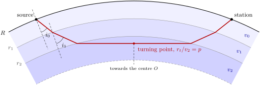
The ray parameter is not only a constant of the ray: it can be read off the travel-time curve.

Theorem 1.3 (Slope of the travel-time curve)

Let $T(\Delta)$ be the travel time of a ray from a surface source to a surface station at the epicentral distance $\Delta$ (in radians). Then

$$\frac{\mathrm dT}{\mathrm d\Delta} = p ,$$

the ray parameter of the ray arriving at $\Delta$.

The theorem is the spherical form of the relation $\mathrm dT/\mathrm dx = 1/c$ between the slope of a travel-time curve and the apparent speed $c$ along the surface. The two functions $T(p)$ and $\Delta(p)$ can be written as integrals over the speed profile.

Proposition 1.4 (Travel time and distance as integrals)

With $\eta = r/v(r)$ decreasing with depth, the ray of parameter $p$ that turns at $r_t$ reaches

$$\Delta(p) = 2\int_{r_t}^{R}\frac{p\,\mathrm dr}{r\sqrt{\eta^2 - p^2}}, \qquad T(p) = 2\int_{r_t}^{R}\frac{\eta^2\,\mathrm dr}{r\sqrt{\eta^2 - p^2}},$$

and the intercept time $\tau(p) = T - p\Delta$ is $\tau(p) = 2\int_{r_t}^{R}\sqrt{\eta^2 - p^2}\,\mathrm dr/r$.

These integrals are how a travel-time table is computed from a model. The ray-tracing script of this chapter does the same sum over 2-km shells of the reference model PREM, and checks it two ways: in a sphere of uniform speed, where the rays are chords and $T = 2R\sin(\Delta/2)/v$ exactly (exercise 5), and against Theorem 1.3, which it does not use.

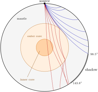
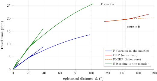
The figure above shows what the theorems predict. The steepest mantle ray that just grazes the core reaches $98.5{}^{\circ}$ in PREM; the next ray, a fraction of a degree steeper, enters the core, is refracted towards the radius and comes out on the far side, beyond $140{}^{\circ}$. Plotting the time against the distance for every ray gives the travel-time curves below.

The computed P times through PREM are $273.5\,\mathrm{s}$ at $20{}^{\circ}$, $369.6\,\mathrm{s}$ at $30{}^{\circ}$, $607.2\,\mathrm{s}$ at $60{}^{\circ}$ and $779.7\,\mathrm{s}$ at $90{}^{\circ}$: thirteen minutes to cross a quarter of the globe.

Real arrivals differ from such a curve by a few seconds at most, and those few seconds are the data of tomography (Section 1.5).

Definition 1.5 (Travel-time table)

A travel-time table gives, for each seismic phase (P, S, PKP, PcP, …) and each source depth, the travel time as a function of epicentral distance, computed from a spherically symmetric reference model whose speeds were themselves adjusted to fit the times of a large set of well-located earthquakes. Its differences from an observed arrival are the starting point of earthquake location and of tomography.

The tables in use today are computed from reference models built for that purpose. In the model ak135, for instance, the crust has two layers, with P and S speeds of 5.80 and $3.46\,\mathrm{km}\,\mathrm{s}^{-1}$ above $20\,\mathrm{km}$ and 6.50 and $3.85\,\mathrm{km}\,\mathrm{s}^{-1}$ down to the Moho at $35\,\mathrm{km}$, where the mantle starts at 8.04 and $4.48\,\mathrm{km}\,\mathrm{s}^{-1}$; the core–mantle boundary lies at $2891.5\,\mathrm{km}$ and the inner-core boundary at $5153.5\,\mathrm{km}$.

Its authors themselves describe its upper mantle as an artificial construct designed to fit the times out to $30{}^{\circ}$: an average, not the structure under any one place.

Proposition 1.6 (Herglotz–Wiechert inversion)

Suppose $\eta = r/v(r)$ decreases strictly with depth over the radii sampled and the travel-time curve $T(\Delta)$ is known, so that $p(\Delta) = \mathrm dT/\mathrm d\Delta$ is known. Then the ray of parameter $p_1$, which reaches the surface at $\Delta_1$, turns at the radius

$$r_1 = R\,\exp\!\left(-\frac1\pi\int_0^{\Delta_1} \operatorname{arccosh}\frac{p(\Delta)}{p_1}\,\mathrm d\Delta\right),$$

where the speed is $v(r_1) = r_1/p_1$. The Herglotz–Wiechert inversion recovers $v(r)$ in this way, point by point, from the travel-time curve.

The formula comes from the integral of $\Delta(p)$ in Proposition 1.4, which is an Abel integral equation for the unknown $r(\eta)$; its inversion is admitted here. Exercise 12 checks it on the uniform sphere. Two conditions limit it. It needs $\eta$ to decrease with depth: a low-velocity layer makes a gap in the travel-time curve, and the inversion cannot see inside the layer. And it needs the whole curve, including the later branches of each triplication, which are hard to pick on a seismogram. These limits are why the reference models are now built by forward modelling and least squares (Section 1.4).

1.2 Surface waves

A free surface traps waves. Near the surface of a half-space, P and S motions in the vertical plane of propagation can combine into a wave that travels along the surface and decays with depth; and where a slow layer lies on faster rock, horizontal shear waves are trapped in the layer by total reflection.

Definition 1.7 (Rayleigh wave, Love wave)

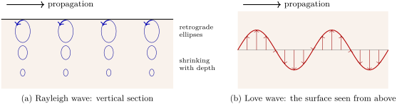
A Rayleigh wave is a surface wave whose particle motion lies in the vertical plane containing the direction of propagation: P and vertically polarised S motions coupled by the free surface, with an elliptical particle motion, retrograde at the surface of a uniform half-space, whose amplitude decays with depth over about a wavelength. A Love wave is a surface wave whose particle motion is horizontal and perpendicular to the direction of propagation: horizontally polarised S waves trapped in layers slower than the rock below them.

On a uniform half-space with $\lambda = \mu$ (a Poisson solid) the Rayleigh wave travels at $0.9194\,\beta$ and does not disperse (exercise 6). A Love wave cannot exist on a uniform half-space at all: it needs the layering, and its speed lies between the S speeds of the layer and of the rock beneath.

Theorem 1.8 (Dispersion of Love waves in a layer over a half-space)

A layer of thickness $H$, shear modulus $\mu_1$ and S speed $\beta_1$ lies on a half-space of shear modulus $\mu_2$ and S speed $\beta_2 > \beta_1$. A Love wave of angular frequency $\omega$ and wave number $k$ propagates with the phase velocity $c = \omega/k$, $\beta_1 < c < \beta_2$, if and only if

$$\tan\!\left(kH q_1\right) = \frac{\mu_2 q_2}{\mu_1 q_1}, \qquad q_1 = \sqrt{\frac{c^2}{\beta_1^2} - 1},\quad q_2 = \sqrt{1 - \frac{c^2}{\beta_2^2}} .$$

The fundamental mode is the root with $0 < kHq_1 < \pi/2$; the overtones have $kHq_1$ in $(n\pi, n\pi + \pi/2)$.

For a given period the equation is solved for $c$ by bisection; the group velocity follows from $U = \mathrm d\omega/\mathrm dk$. At short periods ($kH$ large) the root is near $c = \beta_1$: the wave lives in the layer. At long periods ($kH \to 0$) it must have $kHq_1 \to 0$ with the right-hand side small too, which forces $c \to \beta_2$: the wave reaches deep into the half-space and travels at its speed. Between the two, the phase velocity rises steadily with the period.

Definition 1.9 (Surface-wave dispersion)

Surface-wave dispersion is the dependence of the phase and group velocities of a Rayleigh or Love wave on its period. In a layered Earth it arises because a wave of longer period reaches deeper (about a third of a wavelength for the fundamental mode) and averages faster rock; the dispersion curves $c(T)$ and $U(T)$ measured between an earthquake and a station, or between two stations, are inverted for the S speed as a function of depth.

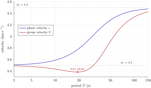
On this model the phase velocity at $20\,\mathrm{s}$ is $3.79\,\mathrm{km}\,\mathrm{s}^{-1}$ and at $100\,\mathrm{s}$ $4.444\,\mathrm{km}\,\mathrm{s}^{-1}$; the group velocities are 3.384 and $4.333\,\mathrm{km}\,\mathrm{s}^{-1}$. On a seismogram recorded a few thousand kilometres away, the long periods arrive first and the 20-s waves last, so that the wave train is drawn out into a long, slowly shortening oscillation. Measuring the group velocity at many periods along many paths gives maps of the crust’s thickness and of the uppermost mantle, independent of the body-wave travel times.

1.3 The Earth rings: normal modes

A surface wave of very long period has a wavelength comparable to the Earth’s radius; it travels round the globe and meets itself. The waves that interfere constructively are the standing waves of the whole sphere, its normal modes, and after a great earthquake they are the last signal to die away. Their theory, an eigenvalue problem for the elastic, self-gravitating Earth, is beyond this chapter; their description is not.

The modes of a spherically symmetric Earth form two families. In the toroidal modes, ${}_nT_\ell$, the motion is horizontal, a twisting of spherical shells against one another, with no change of radius or volume: the standing waves of Love waves. In the spheroidal modes, ${}_nS_\ell$, the motion has radial and horizontal parts, and the Earth changes shape: the standing waves of Rayleigh waves, coupled to the body waves and to gravity. The index $\ell$ is the angular degree, the number of nodal lines of the pattern on the surface; $n$ counts the nodes of the motion with radius, $n = 0$ for the fundamental mode. The gravest spheroidal mode, ${}_0S_2$, stretches the Earth alternately into a prolate and an oblate spheroid; the gravest toroidal mode, ${}_0T_2$, twists the northern and southern hemispheres in opposite directions. Their observed periods are:

Each period is an average over the whole planet of its elastic moduli and density, weighted by where the mode moves: the toroidal modes sense only the solid mantle and crust, the spheroidal modes the core as well. Fitting the periods of hundreds of modes is the only seismological way to weigh the interior: it constrains the density, not only the speeds, and PREM was built to fit them together with the travel times. The rotation and the ellipticity of the Earth split each mode of degree $\ell$ into $2\ell + 1$ slightly different frequencies, the analogue of the Zeeman effect.

History — The Earth after the Chilean earthquake

The 1960 Chilean earthquake was recorded by long-period pendulum seismometers and by strainmeters, instruments that measure the change in length of a long horizontal rod or wire anchored in rock. Spectral analysis of a few days of record showed sharp peaks at the predicted periods of the gravest modes: the whole Earth had been set ringing, and the predictions of the elastic theory of a spherical, self-gravitating Earth were met. The record of the strainmeter at Isabella, in California, was analysed again in 1978 with more modern methods: it showed clearly the splitting of ${}_0T_3$, ${}_0T_4$, ${}_0S_4$ and ${}_0S_5$ by the rotation and ellipticity of the Earth, and confirmed that of ${}_0S_2$ and ${}_0S_3$.

Normal-mode seismology, born of one earthquake, now uses the networks of very-broadband stations that record every great earthquake.

1.4 Linear inverse problems

Every method of this chapter so far computes data from a model. The task of imaging is the reverse.

Definition 1.10 (Forward problem, inverse problem)

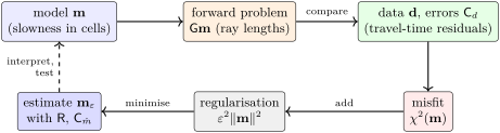
Let a model of the Earth be described by a vector $\mathbf m$ of $M$ parameters and the observations by a vector $\mathbf d$ of $N$ data. The forward problem is to compute the data $\mathbf d = g(\mathbf m)$ that a given model would produce, by a physical theory. The inverse problem is to estimate the model from data that carry errors, $\mathbf d = g(\mathbf m) + \mathbf e$, and to say how well each part of the model is determined. The problem is linear when $g(\mathbf m) = \mathsf G\mathbf m$ for a fixed $N\times M$ matrix $\mathsf G$, the kernel.

Fitting a straight line through travel times is a linear inverse problem with $M = 2$ (exercise 7); a travel-time tomography is one with thousands of parameters. Three cases arise. If $N > M$ and the data constrain every parameter, the problem is overdetermined: no model fits every datum exactly, and the best is sought in a statistical sense. If some combination of parameters leaves the data unchanged ($\mathsf G\mathbf m_0 = \mathbf 0$ for some $\mathbf m_0 \ne \mathbf 0$), the problem is underdetermined in that direction, and no amount of data of that kind will fix it. Real problems are mixed: overdetermined in some parts of the model and underdetermined in others.

Theorem 1.11 (Weighted least-squares estimate)

Let $\mathbf d = \mathsf G\mathbf m + \mathbf e$, where the errors $\mathbf e$ have zero mean and the covariance matrix $\mathsf C_d$ (diagonal $\sigma_i^2$ for independent errors). If the matrix $\mathsf N = \mathsf G^{\mathsf T}\mathsf C_d^{-1}\mathsf G$ is invertible, the model that minimises the misfit

$$\chi^2(\mathbf m) = (\mathbf d - \mathsf G\mathbf m)^{\mathsf T}\mathsf C_d^{-1} (\mathbf d - \mathsf G\mathbf m)$$

is the weighted least-squares estimate

$$\hat{\mathbf m} = \mathsf N^{-1}\mathsf G^{\mathsf T}\mathsf C_d^{-1}\mathbf d ,$$

it is unbiased, and its covariance matrix is $\mathsf C_{\hat m} = \mathsf N^{-1}$.

The weights do what intuition asks: a datum with half the error counts four times as much. The covariance matrix gives each parameter its standard error $\sqrt{(\mathsf N^{-1})_{jj}}$ and the correlations between them. If the model is right and the errors Gaussian, the minimum $\chi^2$ follows a $\chi^2$ law with $N - M$ degrees of freedom: a value far above $N - M$ means the errors were underestimated or the model is too simple; far below, that the errors were overestimated.

When $\mathsf N$ is singular or nearly so, the estimate does not exist or is dominated by noise amplified along the poorly constrained directions. The standard remedy is to ask for a model that fits the data reasonably and is not needlessly large.

Definition 1.12 (Damped least squares, trade-off curve)

For a damping parameter $\varepsilon > 0$, the damped least squares estimate is the model that minimises

$$\Phi_\varepsilon(\mathbf m) = \chi^2(\mathbf m) + \varepsilon^2\|\mathbf m\|^2 , \qquad \mathbf m_\varepsilon = \left(\mathsf N + \varepsilon^2\mathsf I\right)^{-1} \mathsf G^{\mathsf T}\mathsf C_d^{-1}\mathbf d .$$

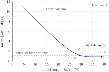
The trade-off curve is the curve traced, as $\varepsilon$ varies, by the pair (size of the model $\|\mathbf m_\varepsilon\|$, misfit $\chi^2(\mathbf m_\varepsilon)$): small damping fits the data closely with a large, rough model, large damping gives a small model and a poor fit.

The formula is found as in Theorem 1.11: the gradient of $\Phi_\varepsilon$ is $-2\mathsf G^{\mathsf T}\mathsf C_d^{-1}(\mathbf d - \mathsf G\mathbf m) + 2\varepsilon^2\mathbf m$, and $\mathsf N + \varepsilon^2 \mathsf I$ is always invertible, since its eigenvalues are those of $\mathsf N$ (all $\ge 0$) increased by $\varepsilon^2$. The damping is usually chosen near the knee of the trade-off curve, or so that $\chi^2$ is about the number of data, the misfit expected from the errors alone. The price is that the estimate is no longer unbiased.

Definition 1.13 (Model resolution matrix)

For a linear estimate $\mathbf m_\varepsilon = \mathsf H_\varepsilon \mathbf d$ of the model $\mathbf m$ from data $\mathbf d = \mathsf G\mathbf m + \mathbf e$, the model resolution matrix is $\mathsf R = \mathsf H_\varepsilon\mathsf G$, so that

$$\mathbf m_\varepsilon = \mathsf R\,\mathbf m + \mathsf H_\varepsilon\mathbf e .$$

For damped least squares, $\mathsf R = (\mathsf N + \varepsilon^2\mathsf I)^{-1} \mathsf N$. Row $j$ of $\mathsf R$ shows how the estimate of parameter $j$ averages the true parameters; $\mathsf R = \mathsf I$ means perfect resolution.

If $\mathsf N$ has the orthonormal eigenvectors $\mathbf u_k$ and eigenvalues $\lambda_k$, then $\mathsf R = \sum_k \frac{\lambda_k}{\lambda_k + \varepsilon^2} \mathbf u_k\mathbf u_k^{\mathsf T}$: the directions the data constrain well ($\lambda_k \gg \varepsilon^2$) pass almost unchanged, those they constrain poorly are suppressed. The trace of $\mathsf R$ counts the parameters the data effectively resolve, and the covariance of the estimate, $\mathsf H_\varepsilon\mathsf C_d\mathsf H_\varepsilon^{\mathsf T}$, shrinks as the resolution does: damping trades resolution for stability.

1.5 Seismic tomography

Definition 1.14 (Seismic tomography, travel-time residual)

The travel-time residual of an arrival is the observed travel time minus the time predicted by a reference model, $\delta t = T_{\text{obs}} - T_{\text{ref}}$, after correction for the source location and origin time, the station’s elevation and the Earth’s ellipticity. Seismic tomography is the estimation of the three-dimensional departures of the seismic speeds from a reference model, $\delta v(\mathbf x)$, from a large set of residuals (or of waveforms), by solving an inverse problem.

Write $s = 1/v$ for the slowness. The travel time along a ray $\Gamma$ is $T = \int_\Gamma s\,\mathrm dl$; but the ray itself depends on the speeds, which seems to make the problem non-linear. The first-order answer is that it does not matter.

Proposition 1.15 (Linearised travel-time residual)

If the slowness of the reference model $s_0$ is perturbed to $s_0 + \delta s$, the travel time between two fixed points changes, to first order in $\delta s$, by

$$\delta t = \int_{\Gamma_0}\delta s\,\mathrm dl ,$$

the integral being taken along the ray $\Gamma_0$ of the reference model; the relative speed anomaly is $\delta v/v_0 = -\delta s/s_0$ to the same order.

Cut the region into $M$ cells of uniform slowness perturbation $\delta s_j$. The residual of ray $i$ becomes $\delta t_i = \sum_j L_{ij}\,\delta s_j$, where $L_{ij}$ is the length of the reference ray $i$ in cell $j$: a linear inverse problem whose kernel is the matrix of ray lengths, almost all of whose entries are zero. The residuals are small: in a mantle at $8\,\mathrm{km}\,\mathrm{s}^{-1}$, a region $200\,\mathrm{km}$ across that is $3\,\%$ faster advances a vertical ray by about $0.7\,\mathrm{s}$ (exercise 9).

Method 1.16 (A travel-time tomography)

1. Pick the arrival times of one phase (say P) at all stations, for earthquakes whose location is well known; compute the residuals against a travel-time table, corrected for ellipticity and station elevation.
2. Trace the reference rays and cut the region into cells (or expand $\delta s$ on smooth functions); fill the matrix of ray lengths.
3. Assign each residual its error, from the picking precision, and solve the damped least-squares problem for a range of damping values; draw the trade-off curve and choose the damping near its knee.
4. Test the resolution: compute the residuals that a known synthetic model would give through the same rays, add noise, invert them with the same damping, and compare.
5. Interpret only the anomalies that the test shows the rays can recover, with their amplitudes understood as lower bounds.

Definition 1.17 (Checkerboard test)

A checkerboard test is a resolution test in which the synthetic model is a regular pattern of alternately fast and slow cells: synthetic residuals computed through the real ray geometry, with noise of the size of the real errors, are inverted with the same parametrisation and damping. Where the pattern is recovered, structures of that size can be resolved; where it is smeared or lost, they cannot.

The figures below run the test on a model section $800\,\mathrm{km}$ wide and $400\,\mathrm{km}$ deep, cut into 128 cells of $50\,\mathrm{km}$. Twenty sources lie along its base and thirty-two stations along its top, and only the rays within $45{}^{\circ}$ of the vertical are used: 480 rays that all travel steeply upwards, the geometry of rays from distant earthquakes rising beneath a network. The synthetic model has blocks of $2\times2$ cells, $3\,\%$ fast or slow around $8\,\mathrm{km}\,\mathrm{s}^{-1}$; the residuals carry Gaussian noise of $0.05\,\mathrm{s}$.

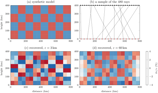
The test illustrates the three limits of every tomographic image. Resolution is set by the rays: where all rays are parallel, an anomaly is smeared along them, and a cell crossed by few rays is barely constrained. Damping lowers the amplitudes: the recovered anomalies are lower bounds. And the image depends on the reference model and the parametrisation: only the departures from the reference are mapped, and nothing smaller than a cell. With these cautions, the global P- and S-wave images show the slabs of the Year 1 volume (in its chapter on subduction) as tabular fast regions descending from the trenches, some flattening above the 670-km discontinuity, others plunging into the lower mantle; and broad slow regions under the Pacific and Africa above the core, with narrower slow conduits beneath some hotspots, the candidates for the mantle plumes of the same volume.

In the field — A broadband station and an ocean-bottom deployment

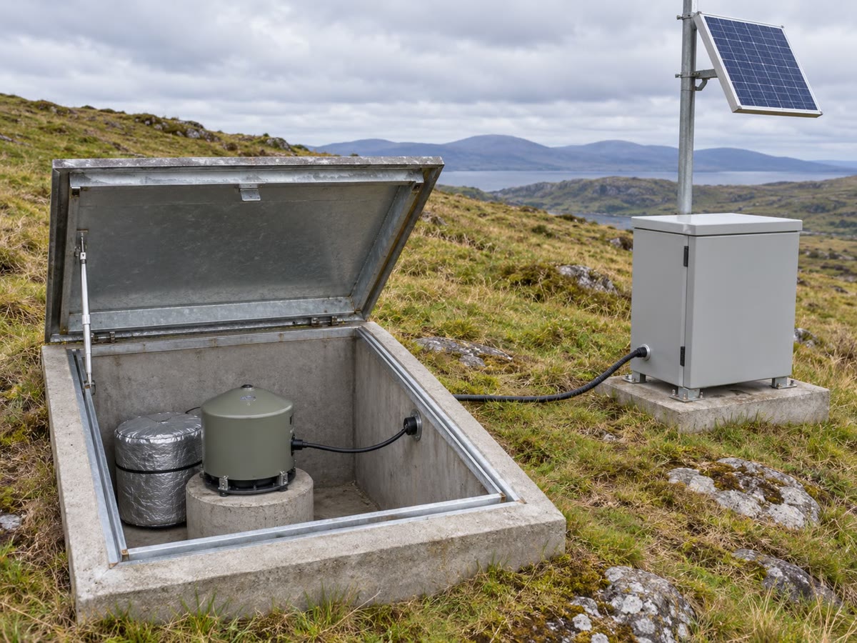
A permanent broadband station is a quiet place: the seismometer stands on a concrete pier bolted to bedrock in a buried vault or a short tunnel, under a thermal shield, because a draught or a change of a few hundredths of a degree tilts the instrument more than a distant earthquake. Its three components, vertical, north and east, are digitised continuously and sent to a data centre with a satellite time stamp. To image a region beneath the ocean, a survey team instead drops ocean-bottom seismometers from a ship: each sinks on an anchor, records for a year on the sea floor, and returns to the surface when the ship comes back and sends an acoustic signal to release it. The crew then reads its clock drift, corrects the records, and adds thousands of arrivals to the tomography.

1.6 Exercises

Exercise 1.1 ★

A P ray leaves the surface ($R = 6371\,\mathrm{km}$, $v_0 = 5.80\,\mathrm{km}\,\mathrm{s}^{-1}$) with the ray parameter $p = 500\,\mathrm{s}\,\mathrm{rad}^{-1}$. (a) Compute its take-off angle. (b) PREM gives P speeds of $11.066\,\mathrm{km}\,\mathrm{s}^{-1}$ at $771\,\mathrm{km}$ depth and $11.245\,\mathrm{km}\,\mathrm{s}^{-1}$ at $871\,\mathrm{km}$. Compute $r/v$ at both depths and find the turning depth of the ray by linear interpolation.

Solution

Solution of Exercise 1.1.

(a) $\sin i_0 = pv_0/R = 500\times5.80/6371 = 0.4552$, so $i_0 = 27.1{}^{\circ}$. (b) At $771\,\mathrm{km}$, $r = 5600\,\mathrm{km}$ and $r/v = 5600/11.066 = 506.1\,\mathrm{s}\,\mathrm{rad}^{-1}$; at $871\,\mathrm{km}$, $r = 5500\,\mathrm{km}$ and $r/v = 5500/11.245 = 489.1\,\mathrm{s}\,\mathrm{rad}^{-1}$. The ray turns where $r/v = p = 500$: $z_t = 771 + 100\times(506.1 - 500)/(506.1 - 489.1) = 771 + 36 = 807\,\mathrm{km}$.

Exercise 1.2 ★

The P times computed through PREM in this chapter are $369.6\,\mathrm{s}$ at $30{}^{\circ}$ and $455.5\,\mathrm{s}$ at $40{}^{\circ}$. (a) Estimate the slope of the travel-time curve between them, in $\mathrm{s}$ per degree and in $\mathrm{s}\,\mathrm{rad}^{-1}$. (b) Deduce the apparent speed of the wave front along the surface, in $\mathrm{km}\,\mathrm{s}^{-1}$. (c) What is the P speed at the turning point of the ray arriving at $35{}^{\circ}$, if it turns at the radius $5450\,\mathrm{km}$?

Solution

Solution of Exercise 1.2.

(a) $(455.5 - 369.6)/10 = 8.59\,\mathrm{s}$ per degree, and $8.59\times180/\pi = 492.2\,\mathrm{s}\,\mathrm{rad}^{-1}$. (b) One degree of arc is $6371\pi/180 = 111.19\,\mathrm{km}$, so the wave front sweeps the surface at $111.19/8.59 = 12.94\,\mathrm{km}\,\mathrm{s}^{-1}$, far faster than any rock at the surface: the ray arrives steeply. (c) At the turning point $v = r_t/p = 5450/492.2 = 11.07\,\mathrm{km}\,\mathrm{s}^{-1}$, a lower-mantle P speed.

Exercise 1.3 ★

In the Love-wave model of this chapter the layer has $\beta_1 = 3.5\,\mathrm{km}\,\mathrm{s}^{-1}$, $\rho_1 = 2700\,\mathrm{kg}\,\mathrm{m}^{-3}$ and the half-space $\beta_2 = 4.5\,\mathrm{km}\,\mathrm{s}^{-1}$, $\rho_2 = 3300\,\mathrm{kg}\,\mathrm{m}^{-3}$. (a) Compute the two shear moduli. (b) At $20\,\mathrm{s}$ the phase velocity is $3.79\,\mathrm{km}\,\mathrm{s}^{-1}$: compute the wavelength and compare it with the layer thickness, $35\,\mathrm{km}$. (c) With group velocities of $3.384\,\mathrm{km}\,\mathrm{s}^{-1}$ at $20\,\mathrm{s}$ and $4.333\,\mathrm{km}\,\mathrm{s}^{-1}$ at $100\,\mathrm{s}$, by how many minutes do the 20-s waves arrive after the 100-s waves at a station $4000\,\mathrm{km}$ away?

Solution

Solution of Exercise 1.3.

(a) $\mu_1 = \rho_1\beta_1^2 = 2700\times3500^2 = 3.31 \times 10^{10}\,\mathrm{Pa}$ ($33.1\,\mathrm{GPa}$); $\mu_2 = 3300\times4500^2 = 6.68 \times 10^{10}\,\mathrm{Pa}$ ($66.8\,\mathrm{GPa}$). (b) $\lambda = cT = 3.79\times20 = 75.8\,\mathrm{km}$, 2.17 times the layer thickness: the wave reaches well into the half-space, which is why its speed is already above $\beta_1$. (c) $4000/3.384 = 1182\,\mathrm{s}$ and $4000/4.333 = 923\,\mathrm{s}$: the 20-s waves arrive $259\,\mathrm{s}$, or $4.3\,\mathrm{min}$, after the 100-s waves.

Exercise 1.4 ★

The observed periods of ${}_0S_2$ and ${}_0T_2$ are $53.89\,\mathrm{min}$ and $44.01\,\mathrm{min}$. (a) Compute their frequencies in $\mathrm{mHz}$. (b) How many oscillations of each does the Earth complete in a day? (c) Two spectral peaks can be separated only if the record lasts at least the inverse of their frequency difference. How long must a record be to separate these two modes?

Solution

Solution of Exercise 1.4.

(a) ${}_0S_2$: $1/(53.89\times60) = 3.093 \times 10^{-4}\,\mathrm{Hz} = 0.3093\,\mathrm{mHz}$; ${}_0T_2$: $1/(44.01\times60) = 0.3787\,\mathrm{mHz}$. (b) $1440/53.89 = 26.7$ and $1440/44.01 = 32.7$ oscillations a day. (c) The difference is $0.0694\,\mathrm{mHz}$, whose inverse is $14\,400\,\mathrm{s}$: at least $4.0\,\mathrm{h}$ of record, in practice much more, since the peaks are broadened by attenuation and split.

Exercise 1.5 ★★

In a sphere of radius $R$ and uniform speed $v$ the rays are straight chords. (a) Show that the ray reaching $\Delta$ has the travel time $T = 2R\sin(\Delta/2)/v$. (b) With $R = 6371\,\mathrm{km}$ and $v = 10.0\,\mathrm{km}\,\mathrm{s}^{-1}$, compute $T$ at $30{}^{\circ}$ and $90{}^{\circ}$, and compare with the PREM times, $369.6\,\mathrm{s}$ and $779.7\,\mathrm{s}$. (c) Explain why the uniform sphere is too fast at $30{}^{\circ}$ and too slow at $90{}^{\circ}$.

Solution

Solution of Exercise 1.5.

(a) The chord between two points of the sphere separated by the angle $\Delta$ at the centre has the length $2R\sin(\Delta/2)$, travelled at $v$. (b) At $30{}^{\circ}$: $2\times6371\times\sin15{}^{\circ}/10.0 = 329.8\,\mathrm{s}$, against $369.6\,\mathrm{s}$; at $90{}^{\circ}$: $2\times6371\times\sin45{}^{\circ}/10.0 = 901.0\,\mathrm{s}$, against $779.7\,\mathrm{s}$. (c) The ray to $30{}^{\circ}$ turns in the upper mantle, where the true speed is about 8 to $10\,\mathrm{km}\,\mathrm{s}^{-1}$, below the uniform $10\,\mathrm{km}\,\mathrm{s}^{-1}$; the ray to $90{}^{\circ}$ spends most of its path in the lower mantle, at 11 to $13.7\,\mathrm{km}\,\mathrm{s}^{-1}$, and bends down into it, so the real Earth is faster.

Exercise 1.6 ★★

On a Poisson solid ($\lambda = \mu$, so $\alpha^2 = 3\beta^2$) the Rayleigh wave speed $c$ satisfies, with $\xi = c^2/\beta^2$, $(2 - \xi)^2 = 4\sqrt{1 - \xi/3}\,\sqrt{1 - \xi}$. (a) Square it and show that the roots satisfy $(\xi - 4)(3\xi^2 - 12\xi + 8) = 0$. (b) Show that the only root with $0 < \xi < 1$ is $\xi = 2 - 2/\sqrt3$, and compute $c/\beta$. (c) In the ak135 upper crust, $\beta = 3.46\,\mathrm{km}\,\mathrm{s}^{-1}$: compute the Rayleigh speed and the delay of the Rayleigh wave behind the S wave at $1000\,\mathrm{km}$.

Solution

Solution of Exercise 1.6.

(a) Squaring, $(2 - \xi)^4 = 16(1 - \xi/3)(1 - \xi)$. Expand: $16 - 32\xi + 24\xi^2 - 8\xi^3 + \xi^4 = 16 - \tfrac{64}{3}\xi + \tfrac{16}{3}\xi^2$, so $\xi^4 - 8\xi^3 + \tfrac{56}{3}\xi^2 - \tfrac{32}{3}\xi = 0$, that is $\xi\,(3\xi^3 - 24\xi^2 + 56\xi - 32) = 0$, and $3\xi^3 - 24\xi^2 + 56\xi - 32 = (\xi - 4)(3\xi^2 - 12\xi + 8)$. The root $\xi = 0$ is not a wave. (b) The roots of the quadratic are $2 \pm 2/\sqrt3$, that is 3.155 and 0.8453; only $\xi = 0.8453$ lies in $(0, 1)$ (and $\xi = 4$ does not), and it satisfies the unsquared equation, both sides being $4/3$. So $c/\beta = \sqrt{0.8453} = 0.9194$. (c) $c = 0.9194\times3.46 = 3.181\,\mathrm{km}\,\mathrm{s}^{-1}$; over $1000\,\mathrm{km}$, $314.4 - 289.0 = 25.3\,\mathrm{s}$ after the S wave.

Exercise 1.7 ★★

Head-wave arrivals at four stations of a refraction line, at 50, 100, 150 and $200\,\mathrm{km}$ from the shot, are 9.0, 15.3, 21.5 and $27.9\,\mathrm{s}$, with errors of 0.1, 0.1, 0.2 and $0.2\,\mathrm{s}$. Fit $T = a + bx$ by weighted least squares: write $\mathsf G$ and $\mathsf C_d$, form the normal equations, and give $a$, $b$, their standard errors, the speed $1/b$ with its error, and the minimum $\chi^2$. Is the fit acceptable?

Solution

Solution of Exercise 1.7.

$\mathsf G$ has the rows $(1, x_i)$ and $\mathsf C_d^{-1} = \operatorname{diag} (100, 100, 25, 25)$ ($\mathrm{s}^{-2}$). The normal equations are

$$\begin{pmatrix} 250 & 23750 \\ 23750 & 2\,812\,500 \end{pmatrix} \begin{pmatrix} a \\ b \end{pmatrix} = \begin{pmatrix} 3665 \\ 418125 \end{pmatrix},$$

with determinant $1.390\,625 \times 10^{8}$. Hence $b = (250\times418125 - 23750\times3665)/1.390\,625 \times 10^{8} = 0.125\,75\,\mathrm{s}\,\mathrm{km}^{-1}$ and $a = (2812500\times3665 - 23750\times418125)/1.390\,625 \times 10^{8} = 2.713\,\mathrm{s}$. The covariance is $\mathsf N^{-1}$: $\sigma_b = \sqrt{250/1.390\,625 \times 10^{8}} = 0.001\,34\,\mathrm{s}\,\mathrm{km}^{-1}$, $\sigma_a = \sqrt{2812500/1.390\,625 \times 10^{8}} = 0.142\,\mathrm{s}$. The speed is $1/b = 7.95\,\mathrm{km}\,\mathrm{s}^{-1}$, with the error $\sigma_b/b^2 = 0.08\,\mathrm{km}\,\mathrm{s}^{-1}$: an uppermost-mantle speed. The residuals are $-0.001$, $0.011$, $-0.076$ and $0.036\,\mathrm{s}$, and $\chi^2 = 0.19$ for $4 - 2 = 2$ degrees of freedom: smaller than expected, so the stated errors are, if anything, generous; the fit is acceptable.

Exercise 1.8 ★★

One ray crosses two cells, with lengths $30\,\mathrm{km}$ and $40\,\mathrm{km}$, and has a residual of $0.50\,\mathrm{s}$. (a) Why is $\mathsf N = \mathsf G^{\mathsf T} \mathsf G$ singular? (b) Among the models that fit the residual exactly, the one of smallest norm is $\mathbf m = \mathsf G^{\mathsf T}(\mathsf G\mathsf G^{\mathsf T})^{-1}\mathbf d$: compute it. (c) Compute the matrix $\mathsf R = \mathsf G^{\mathsf T}(\mathsf G\mathsf G^{\mathsf T})^{-1}\mathsf G$ and its trace. (d) If the true anomaly is $0.01\,\mathrm{s}\,\mathrm{km}^{-1}$ in the first cell only, what is recovered?

Solution

Solution of Exercise 1.8.

(a) $\mathsf G = (30\;\;40)$ is a single row: $\mathsf G^{\mathsf T}\mathsf G$ is $2\times2$ of rank one, hence singular; any model with $30m_1 + 40m_2 = 0$ can be added without changing the datum. (b) $\mathsf G\mathsf G^{\mathsf T} = 900 + 1600 = 2500$, so $\mathbf m = (30, 40)\times0.50/2500 = (0.006, 0.008)\,\mathrm{s}\,\mathrm{km}^{-1}$. (c) $\mathsf R = \frac{1}{2500} \begin{pmatrix} 900 & 1200 \\ 1200 & 1600 \end{pmatrix} = \begin{pmatrix} 0.36 & 0.48 \\ 0.48 & 0.64 \end{pmatrix}$, of trace 1: one datum resolves one combination of parameters. (d) $\mathsf R\,(0.01, 0) = (0.0036, 0.0048)\,\mathrm{s}\,\mathrm{km}^{-1}$: the anomaly is spread along the ray, more into the cell where the ray is longer.

Exercise 1.9 ★★

A slab region of the mantle is $3\,\%$ faster than its surroundings, where $v = 9.0\,\mathrm{km}\,\mathrm{s}^{-1}$. (a) Compute the residual of a ray crossing $200\,\mathrm{km}$ of it vertically, by Proposition 1.15, and exactly. (b) The same for a ray crossing a $100\,\mathrm{km}$ thickness of it at $40{}^{\circ}$ from the normal to the slab. (c) What is the relative error of the linearisation?

Solution

Solution of Exercise 1.9.

(a) Linearised: $\delta t = -(\delta v/v)L/v = -0.03\times200/9.0 = -0.667\,\mathrm{s}$; exactly, $L/(1.03v) - L/v = 200/9.27 - 200/9.0 = -0.647\,\mathrm{s}$. (b) The path in the slab is $100/\cos40{}^{\circ} = 130.5\,\mathrm{km}$: $-0.03\times130.5/9.0 = -0.435\,\mathrm{s}$ linearised and $-0.422\,\mathrm{s}$ exactly. (c) The exact value is the linearised one divided by $1.03$: an error of $3\,\%$, of the order of $\delta v/v$ itself, as expected of a first-order theory.

Exercise 1.10 ★★★

In Theorem 1.8, an overtone of order $n$ exists only at periods short enough. (a) Show that at its cut-off its phase velocity is $\beta_2$ and $kHq_1 = n\pi$. (b) Deduce the cut-off angular frequency $\omega_n = n\pi\beta_1\beta_2/\bigl(H\sqrt{\beta_2^2 - \beta_1^2}\bigr)$. (c) Compute the cut-off period of the first overtone for the chapter’s model ($H = 35\,\mathrm{km}$, $\beta_1 = 3.5$, $\beta_2 = 4.5\,\mathrm{km}\,\mathrm{s}^{-1}$). (d) Show that the fundamental mode has no cut-off, and that its phase velocity tends to $\beta_1$ at short periods.

Solution

Solution of Exercise 1.10.

(a) The overtone exists while its half-space part decays, $c < \beta_2$; at its cut-off $c = \beta_2$, so $q_2 = 0$ and $\tan(kHq_1) = 0$, with $kHq_1$ in $[n\pi, n\pi + \pi/2)$: $kHq_1 = n\pi$. (b) With $k = \omega/\beta_2$ and $q_1 = \sqrt{\beta_2^2/\beta_1^2 - 1} = \sqrt{\beta_2^2 - \beta_1^2}/\beta_1$, $\omega_nH\sqrt{\beta_2^2 - \beta_1^2}/(\beta_1\beta_2) = n\pi$, which is the formula. (c) $\sqrt{4.5^2 - 3.5^2} = \sqrt8 = 2.828$; $\omega_1 = \pi\times3.5\times4.5/(35\times2.828) = 0.4998\,\mathrm{rad}\,\mathrm{s}^{-1}$, a period of $2\pi/0.4998 = 12.57\,\mathrm{s}$: at longer periods only the fundamental mode exists. (d) For $n = 0$ the cut-off frequency is zero: the fundamental mode exists at all periods. At short periods $kH \to \infty$ while $kHq_1$ stays below $\pi/2$, so $q_1 \to 0$ and $c \to \beta_1$.

Exercise 1.11 ★★★

Take the ray of exercise 8, with unit data error. (a) Show that, for any $\varepsilon > 0$, $(\mathsf G^{\mathsf T}\mathsf G + \varepsilon^2\mathsf I)^{-1}\mathsf G^{\mathsf T} = \mathsf G^{\mathsf T}(\mathsf G\mathsf G^{\mathsf T} + \varepsilon^2\mathsf I)^{-1}$. (b) Deduce the damped resolution matrix $\mathsf R_\varepsilon = \mathsf G^{\mathsf T}\mathsf G/(\|\mathbf g\|^2 + \varepsilon^2)$, where $\mathbf g = (30, 40)$, and its trace. (c) Compute the trace and the data residual for $\varepsilon^2 = 0$, 2500 and $10\,000$ (in $\mathrm{km}^{2}$). Describe the trade-off.

Solution

Solution of Exercise 1.11.

(a) $\mathsf G^{\mathsf T}(\mathsf G\mathsf G^{\mathsf T} + \varepsilon^2\mathsf I) = (\mathsf G^{\mathsf T}\mathsf G + \varepsilon^2\mathsf I)\mathsf G^{\mathsf T}$; multiply on the left by $(\mathsf G^{\mathsf T}\mathsf G + \varepsilon^2 \mathsf I)^{-1}$ and on the right by $(\mathsf G\mathsf G^{\mathsf T} + \varepsilon^2\mathsf I)^{-1}$, both invertible for $\varepsilon > 0$. (b) Here $\mathsf G\mathsf G^{\mathsf T} = \|\mathbf g\|^2 = 2500$, a number, so $\mathsf R_\varepsilon = \mathsf G^{\mathsf T}\mathsf G/(2500 + \varepsilon^2)$, of trace $2500/(2500 + \varepsilon^2)$. (c) The predicted datum is $\mathbf g\cdot\mathbf m_\varepsilon = 0.50\times2500/(2500 + \varepsilon^2)$ and the residual $0.50\,\varepsilon^2/(2500 + \varepsilon^2)$. For $\varepsilon^2 = 0$: trace 1, residual 0; for 2500: trace 0.5, residual $0.25\,\mathrm{s}$; for $10\,000$: trace 0.2, residual $0.40\,\mathrm{s}$. More damping gives a smaller model, a poorer resolution and a larger misfit.

Exercise 1.12 ★★★

In the uniform sphere of exercise 5: (a) show by Theorem 1.3 that $p(\Delta) = (R/v)\cos(\Delta/2)$, and check it against the definition of $p$ (the take-off angle of a chord). (b) Show that the ray reaching $\Delta_1$ turns at $r_1 = R\cos(\Delta_1/2)$. (c) Admitting that $\int_0^{\Delta_1}\operatorname{arccosh}\bigl(\cos(\Delta/2) /\cos(\Delta_1/2)\bigr)\,\mathrm d\Delta = \pi\ln\bigl(1/\cos(\Delta_1/2)\bigr)$, show that the Herglotz–Wiechert formula returns $r_1$ and the speed $v$.

Solution

Solution of Exercise 1.12.

(a) By exercise 5, $T = (2R/v)\sin(\Delta/2)$, so $\mathrm dT/\mathrm d\Delta = (R/v)\cos(\Delta/2)$. A chord making the angle $\Delta$ at the centre is the base of an isosceles triangle with apex angle $\Delta$, so it meets the radius at the source at $i_0 = (\pi - \Delta)/2$, and $p = R\sin i_0/v = (R/v)\cos(\Delta/2)$: the same. (b) The turning point is the middle of the chord, at the distance $R\cos(\Delta_1/2)$ from the centre; equivalently $r_1 = p_1v$. (c) Here $p(\Delta)/p_1 = \cos(\Delta/2)/\cos(\Delta_1/2)$, and the formula gives $r_1 = R\exp\bigl(-\ln(1/\cos(\Delta_1/2))\bigr) = R\cos(\Delta_1/2)$, as in (b); the speed is $r_1/p_1 = R\cos(\Delta_1/2)\big/ \bigl((R/v)\cos(\Delta_1/2)\bigr) = v$.

1.7 Problem: The Slab beneath Station K

Problem 1.1

Weekend problem — rays, Love waves and a small tomography beneath an invented station

Station K stands on a continent above a subduction zone. This problem uses its records three ways: rays in its crust, the dispersion of Love waves across it, and a small tomography of the mantle below.

Part I — Rays in a gradient. Over distances short enough to neglect the Earth’s curvature, the P speed beneath K rises linearly with depth, $v(z) = v_0 + gz$, with $v_0 = 5.0\,\mathrm{km}\,\mathrm{s}^{-1}$ and $g = 0.05\,\mathrm{s}^{-1}$ ($z$ in km).

1. In flat layers, Snell’s law keeps $p = \sin i/v$ constant. A ray leaves K with $\sin i_0 = 0.8$: compute $i_0$ and $p$.
2. At what depth does it turn, and what is the speed there?
3. Show that $\mathrm di/\mathrm ds = pg$ along the ray, so that it is an arc of circle; give its radius and the depth of its centre.
4. Compute the horizontal distance $X$ at which the ray returns to the surface.
5. Show that $\mathrm dT = \mathrm di/(g\sin i)$ and compute the travel time $T$ exactly.
6. Compute $X$ and $T$ for $p = 0.15\,\mathrm{s}\,\mathrm{km}^{-1}$, and check that $\Delta T/\Delta X$ between the two rays lies between the two values of $p$.

Part II — Love waves and the crust. The crust under K is a layer of S speed $\beta_1 = 3.5\,\mathrm{km}\,\mathrm{s}^{-1}$ and density $\rho_1 = 2.7\,\mathrm{g}\,\mathrm{cm}^{-3}$ over a mantle with $\beta_2 = 4.5\,\mathrm{km}\,\mathrm{s}^{-1}$, $\rho_2 = 3.3\,\mathrm{g}\,\mathrm{cm}^{-3}$; its thickness $H$ is unknown. Between K and a neighbouring station the Love-wave phase velocity is measured: $3.99\,\mathrm{km}\,\mathrm{s}^{-1}$ at $25\,\mathrm{s}$ and $4.25\,\mathrm{km}\,\mathrm{s}^{-1}$ at $40\,\mathrm{s}$.

7. Compute $\mu_1$ and $\mu_2$ in $\mathrm{GPa}$.
8. At $25\,\mathrm{s}$, compute $k$, $q_1$ and $q_2$.
9. Solve the dispersion equation of the fundamental mode for $H$.
10. Do the same at $40\,\mathrm{s}$. Are the two results consistent?
11. Estimate the group velocity between the two periods as $\Delta\omega/\Delta k$, and compare it with the phase velocities.
12. Compute the wavelength at each period, and explain why the two periods sense the crust and the uppermost mantle in different proportions.

Part III — A tomography in four cells. Below K, a block of mantle $200\,\mathrm{km}$ by $200\,\mathrm{km}$ in a vertical section is cut into four square cells of $100\,\mathrm{km}$: 1 (upper left), 2 (upper right), 3 (lower left) and 4 (lower right); the trench and the ocean lie to the left. The reference speed is $v_0 = 8.0\,\mathrm{km}\,\mathrm{s}^{-1}$. In an idealised experiment six straight rays cross it: A along the upper row (cells 1 and 2), B along the lower row (3 and 4), C down the left column (1 and 3), D down the right column (2 and 4), E along the diagonal through 1 and 4, F along the diagonal through 2 and 3. Their residuals are:

ray	A	B	C	D	E	F
$\delta t$ ($\mathrm{s}$)	$0.16$	$-0.48$	$-0.36$	$0.11$	$-0.15$	$-0.27$
error $\sigma$ ($\mathrm{s}$)	0.05	0.05	0.05	0.05	0.10	0.10

Take the model $\mathbf m$ as the slowness perturbations of the cells in $\mathrm{ms}\,\mathrm{km}^{-1}$ ($1\,\mathrm{ms}\,\mathrm{km}^{-1} = 10^{-3}\,\mathrm{s}\,\mathrm{km}^{-1}$), so that the entries of $\mathsf G$ are the ray lengths in $\mathrm{km}$ divided by 1000.

13. Write $\mathsf G$, a $6\times4$ matrix.
14. Show that $\mathsf N = \mathsf G^{\mathsf T}\mathsf C_d^{-1}\mathsf G$ has the rows $(10, 4, 4, 2)$, $(4, 10, 2, 4)$, $(4, 2, 10, 4)$, $(2, 4, 4, 10)$.
15. Compute $\mathbf b = \mathsf G^{\mathsf T}\mathsf C_d^{-1}\mathbf d$.
16. Check that $(1,1,1,1)$, $(1,-1,-1,1)$, $(1,1,-1,-1)$ and $(1,-1,1,-1)$ are eigenvectors of $\mathsf N$, with eigenvalues 20, 4, 8 and 8, and deduce that $\mathsf N^{-1}$ has the rows $(11, -4, -4, 1)/80$, $(-4, 11, 1, -4)/80$, $(-4, 1, 11, -4)/80$ and $(1, -4, -4, 11)/80$.
17. Compute the weighted least-squares estimate $\hat{\mathbf m}$.
18. Convert it into relative speed anomalies $\delta v/v_0$ in per cent.
19. Give the standard error of each cell in $\mathrm{ms}\,\mathrm{km}^{-1}$ and in per cent, and the correlation between cells 1 and 2, and between cells 1 and 4. Explain their signs.
20. Compute the residuals of the six rays after the fit and the minimum $\chi^2$. Is it consistent with the stated errors?

Part IV — Damping, resolution and the slab.

21. For $\varepsilon^2 = 4$ (in the units of $\mathsf N$), give the eigenvalues of $\mathsf R = (\mathsf N + 4\mathsf I)^{-1}\mathsf N$ and show that $\mathsf R$ has the diagonal $2/3$, the entries $1/12$ between cells that share a row or column ray, and $0$ between cells 1 and 4 and between cells 2 and 3.
22. Compute the damped estimate of cell 3 and its speed anomaly. Why is it smaller than the undamped one?
23. The damped model has $\chi^2 = 15.8$ and norm $2.91\,\mathrm{ms}\,\mathrm{km}^{-1}$; the undamped, $\chi^2 = 0.50$ and $4.24\,\mathrm{ms}\,\mathrm{km}^{-1}$. Which would you keep, and why does this problem not need damping?
24. Read row 3 of the damped $\mathsf R$: with which cells is the estimate of cell 3 blurred?
25. Which cell is fast, and which slow? Interpret the fast cell, below and on the ocean side of K, in terms of the subduction zone.
26. Give the P-velocity anomaly of the slab cell in per cent, with its standard error.

Solution

Solution of Problem 1.1.

1. $i_0 = \arcsin 0.8 = 53.13{}^{\circ}$ and $p = 0.8/5.0 = 0.16\,\mathrm{s}\,\mathrm{km}^{-1}$.

2. The ray turns where $v = 1/p = 6.25\,\mathrm{km}\,\mathrm{s}^{-1}$, that is at $z = (6.25 - 5.0)/0.05 = 25\,\mathrm{km}$.

3. Differentiating $\sin i = pv$ along the ray, $\cos i\,\mathrm di/ \mathrm ds = pg\,\mathrm dz/\mathrm ds = pg\cos i$, so $\mathrm di/\mathrm ds = pg$: the direction turns at a constant rate, the curvature of a circle of radius $1/(pg) = 1/(0.16\times0.05) = 125\,\mathrm{km}$. At the turning point the ray is horizontal at $25\,\mathrm{km}$ depth and the centre lies vertically $125\,\mathrm{km}$ above it: at $z = -100\,\mathrm{km}$, that is $v_0/g$ above the surface, where the extrapolated speed would vanish.

4. At the source the radius of the circle is perpendicular to the ray, so it makes the angle $i_0$ with the horizontal, and the centre lies $125\cos i_0$ away horizontally; by symmetry $X = 2\times125\times\cos i_0 = 2\times125\times0.6 = 150\,\mathrm{km}$, or $X = 2\sqrt{1 - p^2v_0^2}/(pg)$.

5. $\mathrm dT = \mathrm ds/v$ with $\mathrm ds = \mathrm di/(pg)$ and $v = \sin i/p$: $\mathrm dT = \mathrm di/(g\sin i)$. Then

$$T = \frac2g\int_{i_0}^{\pi/2}\frac{\mathrm di}{\sin i} = \frac2g\ln\cot\frac{i_0}2 = \frac2g\operatorname{arccosh}\frac1{pv_0} .$$

Here $\cot(26.57{}^{\circ}) = 2$, so $T = 40\ln2 = 27.73\,\mathrm{s}$.

6. For $p = 0.15$: $pv_0 = 0.75$, $\sqrt{1 - 0.5625} = 0.6614$, $X = 2\times0.6614/0.0075 = 176.4\,\mathrm{km}$ and $T = 40\operatorname{arccosh} (1.3333) = 40\times0.7954 = 31.81\,\mathrm{s}$. Then $\Delta T/\Delta X = 4.08/26.4 = 0.155\,\mathrm{s}\,\mathrm{km}^{-1}$, between 0.15 and 0.16, as $\mathrm dT/\mathrm dX = p$ requires.

7. $\mu_1 = 2700\times3500^2 = 33.1\,\mathrm{GPa}$ and $\mu_2 = 3300\times4500^2 = 66.8\,\mathrm{GPa}$.

8. $k = 2\pi/(cT) = 2\pi/(3.99\times25) = 0.062\,99\,\mathrm{rad}\,\mathrm{km}^{-1}$; $q_1 = \sqrt{(3.99/3.5)^2 - 1} = 0.5474$; $q_2 = \sqrt{1 - (3.99/4.5)^2} = 0.4624$.

9. $\tan(kHq_1) = 66.825\times0.4624/(33.075\times0.5474) = 1.707$; the fundamental mode takes $kHq_1 = \arctan1.707 = 1.041$, so $H = 1.041/(0.06299\times0.5474) = 30.2\,\mathrm{km}$.

10. At $40\,\mathrm{s}$: $k = 2\pi/170 = 0.03696$, $q_1 = 0.6888$, $q_2 = 0.3287$, $\tan(kHq_1) = 0.964$, $kHq_1 = 0.7671$ and $H = 0.7671/(0.03696\times0.6888) = 30.1\,\mathrm{km}$. The two agree within the precision of the phase velocities: the crust is about $30\,\mathrm{km}$ thick.

11. $\omega = 0.2513$ and $0.1571\,\mathrm{rad}\,\mathrm{s}^{-1}$, $k = 0.06299$ and $0.036\,96\,\mathrm{rad}\,\mathrm{km}^{-1}$: $U \approx 0.0942/0.02603 = 3.62\,\mathrm{km}\,\mathrm{s}^{-1}$, less than both phase velocities, as it must be when $c$ increases with the period.

12. $\lambda = 3.99\times25 = 99.8\,\mathrm{km}$ and $4.25\times40 = 170\,\mathrm{km}$. The fundamental mode samples down to a fraction of its wavelength: the 25-s wave lies mostly in the crust, the 40-s wave reaches well into the mantle, so its speed is closer to $\beta_2$. Two periods fixing the same $H$ is a check that the two-layer model is adequate.

13. With the columns for cells 1 to 4 and the rows A to F, in units of $1000\,\mathrm{km}$ ($\sqrt2\times100/1000 = 0.1414$):

$$\mathsf G = \begin{pmatrix} 0.1 & 0.1 & 0 & 0 \\ 0 & 0 & 0.1 & 0.1 \\ 0.1 & 0 & 0.1 & 0 \\ 0 & 0.1 & 0 & 0.1 \\ 0.1414 & 0 & 0 & 0.1414 \\ 0 & 0.1414 & 0.1414 & 0 \end{pmatrix}.$$

14. $\mathsf C_d^{-1} = \operatorname{diag}(400, 400, 400, 400, 100, 100)$. A row or column ray contributes $0.1^2\times400 = 4$, a diagonal ray $0.1414^2\times100 = 2$. Cell 1 is crossed by A, C (4 each) and E (2): 10. Cells 1 and 2 share ray A: 4; cells 1 and 3 share C: 4; cells 1 and 4 share E: 2; and so on by symmetry, which gives the four rows stated.

15. A row or column ray contributes $0.1\times400\,\delta t = 40\, \delta t$ to each of its cells, a diagonal ray $0.1414\times100\,\delta t = 14.14\,\delta t$. Cell 1: $40(0.16 - 0.36) + 14.14\times(-0.15) = -10.12$; cell 2: $40(0.16 + 0.11) + 14.14\times(-0.27) = 6.98$; cell 3: $40(-0.48 - 0.36) + 14.14\times(-0.27) = -37.42$; cell 4: $40(-0.48 + 0.11) + 14.14\times(-0.15) = -16.92$.

16. For $(1,1,1,1)$, each row of $\mathsf N$ sums to 20. For $(1,-1,-1,1)$, row 1 gives $10 - 4 - 4 + 2 = 4$ and the others the same pattern. For $(1,1,-1,-1)$, $10 + 4 - 4 - 2 = 8$, and for $(1,-1,1,-1)$, $10 - 4 + 4 - 2 = 8$. The vectors are orthogonal with norm 2, so $\mathsf N^{-1} = \sum_k \mathbf u_k\mathbf u_k^{\mathsf T}/(4\lambda_k)$; its $(1,1)$ entry is $\tfrac14(\tfrac1{20} + \tfrac14 + \tfrac18 + \tfrac18) = \tfrac{11}{80}$, its $(1,2)$ entry $\tfrac14(\tfrac1{20} - \tfrac14 + \tfrac18 - \tfrac18) = -\tfrac4{80}$, its $(1,4)$ entry $\tfrac14(\tfrac1{20} + \tfrac14 - \tfrac18 - \tfrac18) = \tfrac1{80}$, and so on.

17. $\hat{\mathbf m} = \mathsf N^{-1}\mathbf b$: $\hat m_1 = (11\times(-10.121) - 4\times6.982 - 4\times(-37.418) - 16.921)/80 = -0.081$; likewise $\hat m_2 = 1.844$, $\hat m_3 = -3.706$ and $\hat m_4 = -0.931\,\mathrm{ms}\,\mathrm{km}^{-1}$.

18. $\delta v/v_0 = -v_0\,\delta s = -8.0\times10^{-3}\,\hat m$, in per cent $-0.8\,\hat m$: cell 1 $+0.07$, cell 2 $-1.48$, cell 3 $+2.96$, cell 4 $+0.75\,\%$.

19. Every diagonal entry of $\mathsf N^{-1}$ is $11/80$: each cell has the standard error $\sqrt{0.1375} = 0.371\,\mathrm{ms}\,\mathrm{km}^{-1}$, that is $0.30\,\%$. The correlation of cells 1 and 2 is $-4/11 = -0.36$: they share ray A, and a slowness put in one can be traded against the other. Cells 1 and 4, which share only the less precise diagonal E, are weakly and positively correlated, $+1/11 = +0.09$.

20. The predicted residuals are $0.176$, $-0.464$, $-0.379$, $0.091$, $-0.143$ and $-0.263\,\mathrm{s}$; the residuals after the fit are $-0.016$, $-0.016$, $0.019$, $0.019$, $-0.007$ and $-0.007\,\mathrm{s}$, and $\chi^2 = 0.50$ for $6 - 4 = 2$ degrees of freedom: consistent with the stated errors, if anything on the small side.

21. The eigenvectors are those of $\mathsf N$ and the eigenvalues $\lambda/(\lambda + 4)$: $20/24 = 5/6$, $4/8 = 1/2$, $8/12 = 2/3$ twice. As in question 16, $R_{11} = \tfrac14(\tfrac56 + \tfrac12 + \tfrac23 + \tfrac23) = \tfrac23$; $R_{12} = \tfrac14(\tfrac56 - \tfrac12 + \tfrac23 - \tfrac23) = \tfrac1{12}$; $R_{13} = \tfrac14(\tfrac56 - \tfrac12 - \tfrac23 + \tfrac23) = \tfrac1{12}$; $R_{14} = \tfrac14(\tfrac56 + \tfrac12 - \tfrac23 - \tfrac23) = 0$.

22. Project $\mathbf b$ on the eigenvectors: $\mathbf b\cdot\mathbf u_k/4 = -14.37$, $0.849$, $12.80$ and $-9.40$ for the eigenvalues 20, 4, 8 and 8. The damped estimate divides them by $\lambda + 4$ instead of $\lambda$; for cell 3 (components $1, -1, -1, 1$), $m_3 = -14.37/24 - 0.849/8 - 12.80/12 - 9.40/12 = -2.555\,\mathrm{ms}\,\mathrm{km}^{-1}$, a speed anomaly of $+2.04\,\%$. Damping pulls every component towards zero, most of all the poorly constrained ones.

23. The undamped model, which fits the data to within their errors ($\chi^2 = 0.50$ for 2 degrees of freedom), whereas the damped one misfits them badly ($15.8$). Damping is needed only when $\mathsf N$ is singular or nearly so; here its smallest eigenvalue, 4, is not small, the estimate is stable and its errors are moderate.

24. Row 3 is $(1/12, 0, 2/3, 1/12)$: the damped estimate of cell 3 is two thirds of its true value plus a twelfth of cells 1 and 4, its neighbours along ray C and ray B, and nothing of cell 2.

25. Cell 3, the lower cell on the left, is fast by about $3\,\%$; cell 2 is slow. A cold, dense slab of oceanic lithosphere sinking beneath the continent is faster than the surrounding mantle, so the fast cell, deep and on the ocean side of K, is the slab; the slow cell above it on the other side lies where the mantle wedge is hot.

26. From questions 18 and 19, the P-velocity anomaly of the slab cell is $(3.0 \pm 0.3)\,\%$.