书籍暂未推出简体中文版——当前显示英文版。

University Earth and Space Sciences — Year 3 · 本科三年级

23Hydrogeology

A new well pumps $2160\,\mathrm{m}^{3}$ of water a day from a limestone a few hundred metres below a farm. Nothing happens to the farm’s own well at first. A month later its water stands nearly $2\,\mathrm{m}$ lower, although it is a kilometre away and the pumping station has never drawn a drop from it. The water level round the new well has not fallen uniformly: it has sunk into a cone, and the cone has grown, quickly, through a rock in which the water itself moves a few centimetres a day. This chapter builds the physics that predicts both numbers, the fast spread of the pressure and the slow travel of the water, from one empirical law found in 1856.

You already know

Porosity, permeability, the water table, groundwater, aquifers, springs and wells are in the school books, with the residence time of water and fossil groundwater. Viscosity, Poiseuille’s law for the flow in a tube and the diffusion equation are in the physics books. The error function and the solutions of the diffusion equation that use it are in Chapter 5. The Varden Hills, the series’ invented region, with its sandstone, limestone, shale and chalk, are the region of the exercises since the school books.

23.1 Head and Darcy’s law

Water underground moves from where its mechanical energy per unit weight is high to where it is low. Because it moves slowly, its kinetic energy is negligible, and that energy has two parts: the height of the water and its pressure.

Definition 23.1 (Hydraulic head; hydraulic gradient)

The hydraulic head at a point of the saturated ground is

h = z + \frac{p}{\rho g} ,

the sum of the elevation head $z$ of the point above a datum and the pressure head $p/(\rho g)$ , $p$ being the pressure of the water above the atmospheric pressure. It is the elevation to which water rises in a tube, a piezometer, open only at that point. The hydraulic gradient is $\nabla h$ ; its size between two points a distance $L$ apart along the flow is $\Delta h/L$ .

A piezometer, a tube open only at its screen. The water stands in it at the hydraulic head of the point P: its elevation z plus its pressure head. Here the level in the tube is above the water table, as it is where the water rises towards a spring or a river. — A piezometer, a tube open only at its screen. The water stands in it at the hydraulic head of the point $P$ : its elevation $z$ plus its pressure head. Here the level in the tube is above the water table, as it is where the water rises towards a spring or a river.

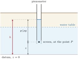
In 1856 Henry Darcy, a French engineer, measured the flow of water through columns of sand and found it proportional to the loss of head per unit length. The flow is laminar: the water follows separate streamlines.

Theorem 23.2 (Darcy’s law)

In a saturated porous medium the volume of water crossing unit area per unit time is

\vec q = -K\,\nabla h ,

where $K$ depends on the medium and on the fluid. In a medium whose pores are parallel straight tubes of radius $a$ occupying a fraction $n$ of the volume, Poiseuille’s law gives this law with

K = \frac{k\rho g}{\mu}, \qquad k = \frac{na^2}{8} ,

$\mu$ being the viscosity of the water.

Proof. The first statement is Darcy’s empirical law. In a tube of radius $a$ along the flow, Poiseuille’s law gives the mean velocity $\bar u = -(a^2/8\mu)\,\mathrm d(p + \rho gz)/\mathrm dl = -(a^2\rho g/8\mu)\,\mathrm dh/\mathrm dl$ , since $p + \rho gz = \rho g h$ . The tubes occupy the fraction $n$ of any cross-section, so the volume per unit total area is $q = n\bar u = -(na^2/8)(\rho g/\mu)\,\mathrm dh/\mathrm dl$ . ∎

Real pores are not straight tubes; the theorem shows the form of the law and how it scales. The flow is proportional to the gradient, to the square of the size of the pores, and inversely to the viscosity: the same sand lets water through faster when it is warm.

Definition 23.3 (Specific discharge; hydraulic conductivity; intrinsic permeability)

The specific discharge $\vec q$ is the volume of water crossing unit area of the medium, grains and pores together, per unit time. The hydraulic conductivity $K$ is the coefficient of Darcy’s law, in $\mathrm{m}/\mathrm{s}$ or $\mathrm{m}/\mathrm{d}$ . The intrinsic permeability of the medium is $k = K\mu/(\rho g)$ , in $\mathrm{m}^{2}$ : it depends on the medium alone.

The hydraulic conductivity of the rocks ranges through twelve orders of magnitude, as few physical quantities do. Read off the chart of a classic survey of the subject, typical ranges, in metres per day, are: clay $10^{-7}$ to $10^{-4}$ ; silt and loess $10^{-3}$ to 2; silty sand 0.04 to 10; clean sand 0.3 to 150; gravel 100 to 4000; shale $10^{-8}$ to $10^{-4}$ ; sandstone $10^{-5}$ to 0.4; carbonate rocks $10^{-4}$ when they are only fractured to several thousand when they are cavernous; igneous and metamorphic rocks below $10^{-8}$ when unfractured to a few when fractured. Most rocks also conduct water better along their bedding than across it.

The specific discharge is a flux through the whole area; the water flows only through the pores, and faster.

Definition 23.4 (Seepage velocity)

The seepage velocity is $\vec v = \vec q/n_e$ , the mean velocity of the water in the pores, $n_e$ being the effective porosity, that of the connected pores through which the water flows.

A coarse sand with $K = 60\,\mathrm{m}/\mathrm{d}$ , a gradient of 1 in 1000 and a porosity of 0.20 moves its water at $0.3\,\mathrm{m}/\mathrm{d}$ ; a clay with $K = 10^{-4}\,\mathrm{m}/\mathrm{d}$ , a gradient of 1 in 10 and a porosity of 0.50, at $2 \times 10^{-5}\,\mathrm{m}/\mathrm{d}$ , less than a centimetre a year. Groundwater does not flow in underground rivers, except in the caves of limestones and the tubes of lavas. These are averages: where a pollutant travels, its fastest part may go several times faster.

23.2 Aquifers

Definition 23.5 (Confined and unconfined aquifers; aquitard)

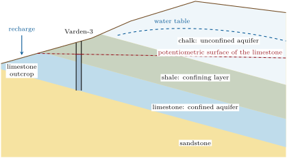
An unconfined aquifer is an aquifer whose upper surface is the water table. A confined aquifer is an aquifer overlain by a layer of much lower conductivity, so that the water in it is under pressure: in a well that reaches it, the water rises above the top of the aquifer, to its potentiometric surface. A layer of low conductivity that slows but does not stop the passage of water between aquifers is an aquitard.

Definition 23.6 (Transmissivity; storativity; specific yield)

The transmissivity of an aquifer of thickness $b$ is $T = Kb$ , the flow per unit width under unit gradient, in $\mathrm{m}^{2}/\mathrm{d}$ . Its storativity (or storage coefficient) $S$ is the volume of water released per unit area of the aquifer when the head falls by one unit; it is dimensionless. The specific yield $S_y$ of a rock is the volume of water that drains from it by gravity per unit volume when the water table falls through it.

The two kinds of aquifer release water in different ways. In a confined aquifer the head falls but the pores stay full: the water expands a little, and the aquifer, carrying more of the weight of the rocks above, is compressed a little. The expansion of the water alone releases about $9 \times 10^{-7}$ cubic metre per cubic metre of aquifer and per metre of head; with the compression, the storativity of most confined aquifers is $10^{-5}$ to $10^{-3}$ . In an unconfined aquifer the water table falls and the pores above it drain: the storativity is the specific yield, about 0.1 to 0.3, a hundred to ten thousand times larger. The transmissivities of the aquifers in use range from less than $1\,\mathrm{m}^{2}/\mathrm{d}$ in fractured rocks to $100\,000\,\mathrm{m}^{2}/\mathrm{d}$ in cavernous limestones and lava flows. Where the head of a confined aquifer is drawn down for a long time, the clays in and around it drain and compact, and the ground above subsides.

A schematic section of the cover of the Varden Hills from west to east, not to scale. The chalk holds an unconfined aquifer below its water table. The Jurassic limestone is recharged where it outcrops and is confined beneath the shale: in the well Varden-3 of the problem, drilled through the shale and open only to the limestone, the water rises to the potentiometric surface, far above the top of the aquifer but below the ground.

23.3 The groundwater-flow equation

Theorem 23.7 (Groundwater-flow equation)

In a confined aquifer of constant transmissivity $T$ and storativity $S$ , with horizontal flow, the head $h(x, y, t)$ obeys

S\,\frac{\partial h}{\partial t} = T\nabla^2h + W ,

$W$ being the volume of water added per unit area and time by recharge or removed by pumping (negative). In steady flow without sources, $\nabla^2h = 0$ .

Proof. Take a column of the aquifer of area $\mathrm dx\,\mathrm dy$ . The flow per unit width through its full thickness is $-T\nabla h$ , by Darcy’s law times $b$ . The net inflow is $-\nabla\cdot(-T\nabla h)\,\mathrm dx\,\mathrm dy = T\nabla^2h\,\mathrm dx\,\mathrm dy$ . The water stored in the column changes at the rate $S\,(\partial h/\partial t)\,\mathrm dx\,\mathrm dy$ , by the definition of $S$ . Mass conservation, the water’s density being treated as constant in the balance, equates storage to inflow plus sources. ∎

It is the diffusion equation of the physics books, with the hydraulic diffusivity $T/S$ in place of a thermal one. For a confined limestone with $T = 450\,\mathrm{m}^{2}/\mathrm{d}$ and $S = 2 \times 10^{-4}$ the diffusivity is $2.25 \times 10^{6}\,\mathrm{m}^{2}/\mathrm{d}$ : a change of head spreads across $1\,\mathrm{km}$ in about $L^2S/T$ , half a day. The same limestone, unconfined, with $S = 0.2$ , would take a thousand times longer. The pressure spreads fast, the water moves slowly: the two numbers of the opening.

Proposition 23.8 (Steady radial flow to a well)

A well pumps $Q$ from a confined aquifer of transmissivity $T$ , the flow being steady and radial. Between two distances $r_1 < r_2$ from the well the drawdowns differ by

s_1 - s_2 = \frac{Q}{2\pi T}\ln\frac{r_2}{r_1} .

Proof. Through every circle of radius $r$ round the well the inflow is $Q = 2\pi r T\,\mathrm dh/\mathrm dr$ . Integrating $\mathrm dh = (Q/2\pi T)\,\mathrm dr/r$ from $r_1$ to $r_2$ , and writing $s = h_0 - h$ , gives the result. ∎

In two dimensions, steady flow is drawn with a flow net.

Definition 23.9 (Flow net)

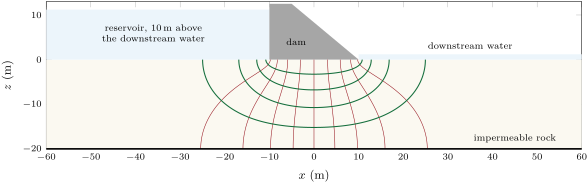
A flow net is a drawing of steady groundwater flow in a homogeneous, isotropic section by two families of curves: equipotentials, lines of equal head, and streamlines, which the water follows. The streamlines cross the equipotentials at right angles, and in a flow net they are spaced so that the cells are curvilinear squares.

Method 23.10 (Seepage from a flow net)

Draw the boundaries: an impermeable boundary is a streamline; a water body’s bed, where the head is fixed, is an equipotential.
Draw $N_d$ head drops between the highest and lowest heads, $\Delta h = H/N_d$ , and the streamlines forming $N_f$ flow channels, by trial, until every cell is a curvilinear square.
Each channel carries $K\Delta h$ per unit length normal to the section, the square’s length and width cancelling: the total is $q = KHN_f/N_d$ .

Seepage under a dam 20\, m wide on a layer of sand 20\, m thick, the reservoir 10\, m above the water downstream, computed by solving Laplace’s equation for the head and for the stream function. Thin lines: equipotentials, one every metre of head. Thick lines: four streamlines which, with the dam base and the floor, bound five flow channels. The computed seepage is 0.51\,KH per metre of dam; the flow net gives KH × 5/10 = 0.50\,KH. — Seepage under a dam $20\,\mathrm{m}$ wide on a layer of sand $20\,\mathrm{m}$ thick, the reservoir $10\,\mathrm{m}$ above the water downstream, computed by solving Laplace’s equation for the head and for the stream function. Thin lines: equipotentials, one every metre of head. Thick lines: four streamlines which, with the dam base and the floor, bound five flow channels. The computed seepage is $0.51\,KH$ per metre of dam; the flow net gives $KH \times 5/10 = 0.50\,KH$ .

23.4 Pumping tests

Steady flow to a well is rare: a new steady state may take months or years, or never come. In 1935 Theis, of the United States Geological Survey, gave the drawdown round a well pumped at a constant rate as a function of time, from which a test of a few hours or days yields the transmissivity and the storativity of the aquifer.

Theorem 23.11 (Theis solution)

A well fully penetrating an infinite, homogeneous, confined aquifer of transmissivity $T$ and storativity $S$ starts at $t = 0$ to pump at the constant rate $Q$ . The drawdown at the distance $r$ is

s(r, t) = \frac{Q}{4\pi T}\,W(u), \qquad u = \frac{r^2S}{4Tt}, \qquad W(u) = \int_u^\infty\frac{\mathrm e^{-y}}{y}\,\mathrm dy = -\gamma - \ln u + u - \frac{u^2}{2\cdot2!} + \frac{u^3}{3\cdot3!} - \cdots,

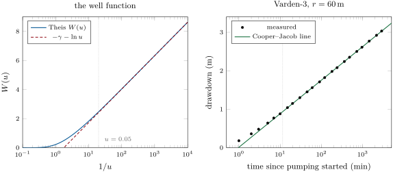
with $\gamma = 0.5772$ . $W$ is called the well function.

Proof. In radial form the flow equation is $S\,\partial s/\partial t = T\,r^{-1}\partial_r(r\,\partial_rs)$ , with $s = 0$ at $t = 0$ , $s \to 0$ as $r \to \infty$ and $2\pi rT\,\partial_rs \to -Q$ as $r \to 0$ . None of the data contains a length or a time on its own, so try $s = f(u)$ with $u = r^2S/4Tt$ . Since $\partial_ru = 2u/r$ and $\partial_tu = -u/t$ , $r\,\partial_rs = 2uf'$ , $r^{-1}\partial_r(r\,\partial_rs) = (4u/r^2)(uf')'$ and $\partial_ts = -(u/t)f'$ . Multiplying the equation by $r^2/(4Tu)$ leaves $(uf')' = -uf'$ : with $g = uf'$ , $g' = -g$ and $g = c\,\mathrm e^{-u}$ . The well condition, $2\pi T\cdot2uf' \to -Q$ as $u \to 0$ , gives $c = -Q/4\pi T$ , and $f(\infty) = 0$ gives $f(u) = (Q/4\pi T)\int_u^\infty \mathrm e^{-y}y^{-1}\,\mathrm dy$ . The series follows from $W(u) = -\gamma - \ln u + \int_0^u(1 - \mathrm e^{-y})\,y^{-1}\,\mathrm dy$ , the constant being Euler’s, by integrating term by term. ∎

Proposition 23.12 (Cooper–Jacob approximation)

When $u \le 0.05$ , the Theis drawdown is close to

s = \frac{2.3\,Q}{4\pi T}\log_{10}\frac{2.25\,Tt}{r^2S} :

plotted against $\log_{10}t$ , the drawdown is a straight line whose rise per log cycle, $\Delta s$ , gives $T = 2.3\,Q/(4\pi\Delta s)$ , and whose intercept with $s = 0$ , at $t_0$ , gives $S = 2.25\,Tt_0/r^2$ .

Proof. For small $u$ the series is $W \approx -\gamma - \ln u = \ln(\mathrm e^{-\gamma}/u) = \ln(0.5615\cdot4Tt/r^2S) = \ln(2.25\,Tt/r^2S)$ ; the next term, $u$ , is at most $0.05$ , under $2\,\%$ of $W$ there. Since $\ln x = 2.3\log_{10}x$ , the drawdown rises by $2.3\,Q/4\pi T$ per factor ten of time, and vanishes when $2.25\,Tt_0 = r^2S$ . ∎

Left, the Theis well function against 1/u on a logarithmic axis, and its straight-line approximation: they merge once u < 0.05 (dotted). Right, the drawdown recorded in the observation well of the Varden-3 test of the problem, 60\, m from the pumped well, and the straight line fitted to the points after 11.5\, min, where u < 0.05: its slope gives T, its intercept S. — Left, the Theis well function against $1/u$ on a logarithmic axis, and its straight-line approximation: they merge once $u < 0.05$ (dotted). Right, the drawdown recorded in the observation well of the Varden-3 test of the problem, $60\,\mathrm{m}$ from the pumped well, and the straight line fitted to the points after $11.5\,\mathrm{min}$ , where $u < 0.05$ : its slope gives $T$ , its intercept $S$ .

Definition 23.13 (Cone of depression)

The cone of depression of a pumped well is the depression of the water table, or of the potentiometric surface, round the well; the gradient steepens towards the well, through which all the water must pass.

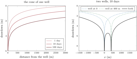
Because the drawdowns obey a linear equation, the cones of several wells add. In a confined aquifer, with its small storativity, a cone grows fast and the cones of neighbouring wells soon interfere; in an unconfined aquifer, which must drain its pores, the cone grows slowly. The cone stops growing only when it has captured enough recharge, or reduced enough of the aquifer’s natural discharge to rivers and springs, to balance the pumping. Large withdrawals from a confined aquifer reach far: in 1981 about $277\,000\,\mathrm{m}^{3}/\mathrm{d}$ pumped from the Cretaceous aquifer of the Atlantic coastal plain, in Virginia and North Carolina, had drawn overlapping cones across it.

The Theis cone of the Varden-3 well (Q = 2160\, m3/ d, T = 450\, m2/ d, S = 2 × 10-4), drawdown plotted downward. Left, after 1, 10 and 100 days: the cone deepens by the same amount for every tenfold time and widens without limit in an infinite aquifer. Right, two such wells 400\, m apart after 10 days: the drawdowns add, 5.5\, m midway between them instead of 2.7\, m for one well. — The Theis cone of the Varden-3 well ( $Q = 2160\,\mathrm{m}^{3}/\mathrm{d}$ , $T = 450\,\mathrm{m}^{2}/\mathrm{d}$ , $S = 2 \times 10^{-4}$ ), drawdown plotted downward. Left, after 1, 10 and 100 days: the cone deepens by the same amount for every tenfold time and widens without limit in an infinite aquifer. Right, two such wells $400\,\mathrm{m}$ apart after 10 days: the drawdowns add, $5.5\,\mathrm{m}$ midway between them instead of $2.7\,\mathrm{m}$ for one well.

In the field — A pumping test

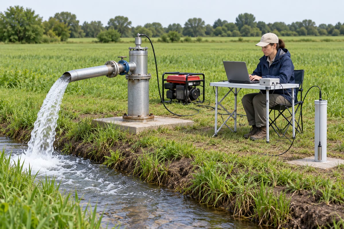
A pumping test: the discharge pipe of the pumped well, a generator, and a hydrogeologist logging the levels of an observation well on a laptop (AI-generated illustration).

Before a pumping test the hydrogeologists record the water levels in the wells for some time, to know the trend that the test will be superimposed on. The pump then runs at a constant rate, held steady and measured by a meter on the discharge pipe, for several hours to several days. In each observation well, at least three of them at different distances if possible, the depth to water below a fixed measuring point is read at precisely known times, many in the first minutes and fewer later: with a graduated steel tape, or an electric tape whose electrode closes a circuit on touching the water. Today a submersible pressure transducer hung in the well, connected to an electronic recorder, logs the level almost continuously.

23.5 Solute transport

A solute dissolved in groundwater is carried with the water, at the seepage velocity, and it spreads as it goes: the water in neighbouring pores moves at different speeds and along different paths, and the solute also diffuses.

Definition 23.14 (Hydrodynamic dispersion; dispersivity)

Hydrodynamic dispersion is the spreading of a solute in flowing groundwater by the variations of the velocity of the water from pore to pore and by molecular diffusion. Along the flow it is described by a dispersion coefficient $D = \alpha_Lv + D^*$ , $v$ the seepage velocity, $D^*$ the effective molecular diffusivity, and $\alpha_L$ , a length, the longitudinal dispersivity of the medium.

Theorem 23.15 (Advection–dispersion equation)

Along a one-dimensional flow of constant seepage velocity $v$ , the concentration $C(x, t)$ of a non-reacting solute obeys

\frac{\partial C}{\partial t} = D\,\frac{\partial^2C}{\partial x^2} - v\,\frac{\partial C}{\partial x} .

If the concentration is held at $C_0$ at $x = 0$ from $t = 0$ , in a medium initially free of solute,

\frac{C}{C_0} = \frac12\left[\operatorname{erfc}\frac{x - vt}{2\sqrt{Dt}} + \mathrm e^{vx/D}\operatorname{erfc}\frac{x + vt}{2\sqrt{Dt}}\right] .

Proof. In a slice of unit cross-section and length $\mathrm dx$ , of effective porosity $n_e$ , the solute stored is $n_eC\,\mathrm dx$ . Its flux is $n_e(vC - D\,\partial C/\partial x)$ , carried with the water and spread by dispersion as Fick’s law spreads a diffusing substance. Conservation gives $n_e\partial_tC = -\partial_x[n_e(vC - D\partial_xC)]$ , the equation. That the formula satisfies it and the conditions is admitted here; Exercise 23.12 checks its spreading. ∎

In the frame moving with the water, $\xi = x - vt$ , the equation is the diffusion equation, and the front spreads as $\sqrt{2Dt} = \sqrt{2\alpha_L vt} = \sqrt{2\alpha_Lx}$ : the width of the front grows as the square root of the distance travelled.

Definition 23.16 (Retardation factor)

A solute that is adsorbed on the grains, in equilibrium and in proportion to its concentration, travels more slowly than the water. Its retardation factor is

R = 1 + \frac{\rho_bK_d}{n} ,

$\rho_b$ being the dry bulk density of the medium, $n$ its porosity and $K_d$ the distribution coefficient, the adsorbed mass per unit mass of solid divided by the concentration in the water. The solute moves at $v/R$ and disperses with $D/R$ .

A solute injected continuously at x = 0 into a flow of seepage velocity 0.5\, m/ d. Left, the concentration 100\, m down-gradient against time: the water itself arrives after 200 days (dotted); the larger the dispersivity, the earlier the first traces and the later the full concentration. An adsorbed solute with R = 3 arrives three times later. Right, the concentration along the flow after 150 days, when the water has travelled 75\, m (dotted). — A solute injected continuously at $x = 0$ into a flow of seepage velocity $0.5\,\mathrm{m}/\mathrm{d}$ . Left, the concentration $100\,\mathrm{m}$ down-gradient against time: the water itself arrives after 200 days (dotted); the larger the dispersivity, the earlier the first traces and the later the full concentration. An adsorbed solute with $R = 3$ arrives three times later. Right, the concentration along the flow after 150 days, when the water has travelled $75\,\mathrm{m}$ (dotted).

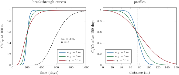
Dispersivities are hard to measure, and in practice they are often set by rules of thumb. The oldest takes the longitudinal dispersivity as a tenth of the length of the plume. A compilation of field measurements published in 1992 shows that the dispersivity grows with the scale of the experiment, that reliable values at large scales are few, and that at any one scale the values spread over two or three orders of magnitude.

23.6 Exercises

Exercise 23.1 ★

Two piezometers stand side by side on ground at $120.0\,\mathrm{m}$ above the datum. The first is screened at $40\,\mathrm{m}$ depth and its water stands $12.5\,\mathrm{m}$ below the ground; the second is screened at $80\,\mathrm{m}$ depth, its water $15.0\,\mathrm{m}$ below the ground. Compute the elevation head, pressure head and hydraulic head at both screens. Which way does the water flow between them, and under what vertical gradient?

Solution

Solution of Exercise 23.1.

First screen: $z = 120 - 40 = 80\,\mathrm{m}$ , $h = 120 - 12.5 = 107.5\,\mathrm{m}$ , pressure head $107.5 - 80 = 27.5\,\mathrm{m}$ . Second screen: $z = 40\,\mathrm{m}$ , $h = 105.0\,\mathrm{m}$ , pressure head $65.0\,\mathrm{m}$ . The head is higher at the shallow screen, so the water flows downward, under a gradient $(107.5 - 105.0)/40 = 0.0625$ : the piezometers stand in a recharge area. The pressure alone would have suggested the opposite.

Exercise 23.2 ★

A column of sand $50\,\mathrm{cm}$ long and $10\,\mathrm{cm}$ in diameter, with $K = 12\,\mathrm{m}/\mathrm{d}$ and an effective porosity of 0.35, carries water under a head difference of $30\,\mathrm{cm}$ . Compute the specific discharge, the flow in litres per hour, and the seepage velocity.

Solution

Solution of Exercise 23.2.

$q = K\Delta h/L = 12\times0.30/0.50 = 7.2\,\mathrm{m}/\mathrm{d}$ . The area is $\pi\times0.05^2 = 7.85 \times 10^{-3}\,\mathrm{m}^{2}$ , so $Q = 0.0565\,\mathrm{m}^{3}/\mathrm{d}$ , or $56.5/24 = 2.36\,\mathrm{L}/\mathrm{h}$ . The seepage velocity is $7.2/0.35 = 20.6\,\mathrm{m}/\mathrm{d}$ .

Exercise 23.3 ★

A limestone has $K = 2.5\,\mathrm{m}/\mathrm{d}$ for water at $10\,{}^{\circ}\mathrm{C}$ ( $\rho = 999.7\,\mathrm{kg}/\mathrm{m}^{3}$ , $\mu = 1.306 \times 10^{-3}\,\mathrm{Pa}\,\mathrm{s}$ ). Compute its intrinsic permeability, and its hydraulic conductivity for water at $20\,{}^{\circ}\mathrm{C}$ ( $\rho = 998.2\,\mathrm{kg}/\mathrm{m}^{3}$ , $\mu = 1.002 \times 10^{-3}\,\mathrm{Pa}\,\mathrm{s}$ ).

Solution

Solution of Exercise 23.3.

$K = 2.5/86400 = 2.894 \times 10^{-5}\,\mathrm{m}/\mathrm{s}$ , and $k = K\mu/(\rho g) = 2.894 \times 10^{-5}\times1.306 \times 10^{-3}/(999.7\times9.81) = 3.85 \times 10^{-12}\,\mathrm{m}^{2}$ . At $20\,{}^{\circ}\mathrm{C}$ , $K$ is multiplied by $(998.2/1.002 \times 10^{-3})/(999.7/1.306 \times 10^{-3}) = 1.30$ : $K = 3.25\,\mathrm{m}/\mathrm{d}$ . The change is almost entirely the viscosity’s.

Exercise 23.4 ★

The confined limestone of Varden-3 is $180\,\mathrm{m}$ thick, with $K = 2.5\,\mathrm{m}/\mathrm{d}$ . Compute its transmissivity, and the storativity it would have if only the expansion of the water, $9 \times 10^{-7}$ per metre of aquifer per metre of head, released water. Compare with $S = 2 \times 10^{-4}$ .

Solution

Solution of Exercise 23.4.

$T = 2.5\times180 = 450\,\mathrm{m}^{2}/\mathrm{d}$ . The expansion of the water gives $9 \times 10^{-7}\times180 = 1.62 \times 10^{-4}$ , about $80\,\%$ of $S = 2 \times 10^{-4}$ ; the compression of the limestone supplies the rest.

Exercise 23.5 ★★

After a long period of pumping at $1500\,\mathrm{m}^{3}/\mathrm{d}$ , the drawdowns have stopped changing: $2.35\,\mathrm{m}$ in an observation well $20\,\mathrm{m}$ from the pumped well and $0.82\,\mathrm{m}$ in one $200\,\mathrm{m}$ away. The aquifer is confined and $40\,\mathrm{m}$ thick. Compute its transmissivity and hydraulic conductivity.

Solution

Solution of Exercise 23.5.

By Proposition 23.8, $T = Q\ln(r_2/r_1)/(2\pi(s_1 - s_2)) = 1500\times\ln10/(2\pi\times1.53) = 359\,\mathrm{m}^{2}/\mathrm{d}$ , and $K = 359/40 = 9.0\,\mathrm{m}/\mathrm{d}$ .

Exercise 23.6 ★★

A well pumps $1200\,\mathrm{m}^{3}/\mathrm{d}$ from a confined aquifer with $T = 300\,\mathrm{m}^{2}/\mathrm{d}$ and $S = 5 \times 10^{-4}$ . Compute $u$ , $W(u)$ (from the series) and the drawdown $300\,\mathrm{m}$ away after 1 day and after 10 days.

Solution

Solution of Exercise 23.6.

$Q/4\pi T = 1200/(4\pi\times300) = 0.318\,\mathrm{m}$ . After 1 day, $u = 300^2\times5 \times 10^{-4}/(4\times300\times1) = 0.0375$ and $W = -0.5772 + 3.2834 + 0.0375 - 0.0004 = 2.743$ : $s = 0.873\,\mathrm{m}$ . After 10 days, $u = 0.003\,75$ , $W = -0.5772 + 5.5860 + 0.0038 = 5.013$ : $s = 1.596\,\mathrm{m}$ . Ten times longer gives less than twice the drawdown.

Exercise 23.7 ★★

For the Varden-3 test ( $T = 450\,\mathrm{m}^{2}/\mathrm{d}$ , $S = 2 \times 10^{-4}$ ), after how many minutes may the Cooper–Jacob line be used in observation wells $60\,\mathrm{m}$ and $500\,\mathrm{m}$ from the pumped well? What does this say about where the observation wells of a short test should be?

Solution

Solution of Exercise 23.7.

$u \le 0.05$ when $t \ge r^2S/(4T\times0.05)$ . At $60\,\mathrm{m}$ : $3600\times 2 \times 10^{-4}/90 = 0.008\,\mathrm{d}$ , $11.5\,\mathrm{min}$ . At $500\,\mathrm{m}$ : $0.556\,\mathrm{d}$ , $800\,\mathrm{min}$ , over 13 hours. The time grows as $r^2$ : in a test of a day or two, the observation wells used for the straight line must be within a few hundred metres of the pumped well.

Exercise 23.8 ★★

Two wells $400\,\mathrm{m}$ apart in the Varden limestone each pump $2160\,\mathrm{m}^{3}/\mathrm{d}$ . Compute the drawdown after 10 days midway between them, and at the second well’s site due to the first well alone. Why does the pumping of each well cost the other money?

Solution

Solution of Exercise 23.8.

Midway, each well is $200\,\mathrm{m}$ away: $u = 200^2\times2 \times 10^{-4}/(4 \times450\times10) = 4.44 \times 10^{-4}$ , $W = 7.142$ , $s = 0.382\times 7.142 = 2.728\,\mathrm{m}$ from each, $5.456\,\mathrm{m}$ in all. At $400\,\mathrm{m}$ , $u = 1.78 \times 10^{-3}$ , $W = 5.757$ , $s = 2.199\,\mathrm{m}$ . Each well lowers the water in the other by $2.2\,\mathrm{m}$ : its pump must lift the water $2.2\,\mathrm{m}$ higher, which costs energy, and the drawdown left before the pump intake runs dry is smaller.

Exercise 23.9 ★★

In the flow net under the dam, count the flow channels and the head drops. With $K = 5\,\mathrm{m}/\mathrm{d}$ and $H = 10\,\mathrm{m}$ , compute the seepage per metre of dam and under a dam $300\,\mathrm{m}$ long.

Solution

Solution of Exercise 23.9.

Four streamlines between the dam base and the floor bound $N_f = 5$ channels; nine equipotentials divide the $10\,\mathrm{m}$ into $N_d = 10$ drops. $q = KHN_f/N_d = 5\times10\times5/10 = 25\,\mathrm{m}^{3}/\mathrm{d}$ per metre of dam, and $7500\,\mathrm{m}^{3}/\mathrm{d}$ under $300\,\mathrm{m}$ . The computed shape factor, 0.512 instead of 0.5, would give $25.6\,\mathrm{m}^{3}/\mathrm{d}$ per metre.

Exercise 23.10 ★★★

Model a clean sand as straight tubes of radius $50\,\text{µ}\mathrm{m}$ with a porosity of 0.30. Compute $k$ and $K$ (for water at $20\,{}^{\circ}\mathrm{C}$ , as in Exercise 23.3), and compare with the range for clean sand. Which features of a real sand does the model leave out, and in which direction does each move $K$ ?

Solution

Solution of Exercise 23.10.

$k = na^2/8 = 0.30\times(5 \times 10^{-5})^2/8 = 9.4 \times 10^{-11}\,\mathrm{m}^{2}$ , and $K = k\rho g/\mu = 9.375 \times 10^{-11}\times998.2\times9.81/1.002 \times 10^{-3} = 9.2 \times 10^{-4}\,\mathrm{m}/\mathrm{s}$ , $79\,\mathrm{m}/\mathrm{d}$ , inside the range of clean sand, 0.3 to $150\,\mathrm{m}/\mathrm{d}$ . The model leaves out the tortuosity of the paths, longer than the straight tubes (it lowers $K$ ), the throats between the pores, narrower than the pores (lower), the pores that end blind and carry no flow (lower), and the spread of the pore sizes: since a tube carries a flow in proportion to $a^4$ , the widest paths carry most of the water and a spread raises $K$ above that of tubes of the mean size.

Exercise 23.11 ★★★

(a) Show that the Cooper–Jacob drawdown vanishes at $r_0 = \sqrt{2.25\,Tt/S}$ . (b) Compute $r_0$ after 30 days of pumping in the confined Varden limestone, and for the same rock unconfined, with $S = 0.2$ . (c) Why can the cone of a confined aquifer reach a boundary that the test was not meant to see?

Solution

Solution of Exercise 23.11.

(a) The logarithm vanishes when $2.25\,Tt = r^2S$ , i.e. at $r_0 = \sqrt{2.25\,Tt/S}$ . (b) Confined and unconfined:

r_0 = \sqrt{\frac{2.25\times450\times30}{2 \times 10^{-4}}} = 12.3\,\mathrm{km}, \qquad r_0 = \sqrt{\frac{2.25\times450\times30}{0.2}} = 390\,\mathrm{m},

$\sqrt{1000} = 31.6$ times smaller. (c) The pressure spreads with the diffusivity $T/S$ , enormous when $S$ is small: within the test the cone reaches faults, the outcrops of the aquifer and rivers, and the drawdown leaves the straight line, which tells the hydrogeologist that a boundary has been met.

Exercise 23.12 ★★★

(a) For a long travel distance the breakthrough curve at $x$ is close to a normal distribution in time, of mean $x/v$ and standard deviation $\sigma_t = \sqrt{2\alpha_Lx}/v$ . Show it from the spreading $\sqrt{2Dt}$ of the front. (b) At $100\,\mathrm{m}$ , with $v = 0.5\,\mathrm{m}/\mathrm{d}$ , the concentration reaches $16\,\%$ after $152.6$ days and $84\,\%$ after $247.2$ days. Estimate $\alpha_L$ . (c) A sandy aquifer has $\rho_b = 1.9\,\mathrm{g}/\mathrm{cm}^{3}$ and $n = 0.30$ ; a solute has $K_d = 0.32\,\mathrm{cm}^{3}/\mathrm{g}$ . Compute $R$ .

Solution

Solution of Exercise 23.12.

(a) Seen from the frame moving with the water, the front is spread with standard deviation $\sigma_x = \sqrt{2Dt} = \sqrt{2\alpha_Lvt}$ . It passes $x$ around $t = x/v$ , when $\sigma_x = \sqrt{2\alpha_Lx}$ ; at the speed $v$ , a spread of $\sigma_x$ in distance is one of $\sigma_t = \sigma_x/v$ in time. (b) The $16\,\%$ and $84\,\%$ times lie one standard deviation either side of the mean: $\sigma_t = (247.2 - 152.6)/2 = 47.3\text{ days}$ . Then $\alpha_L = v^2\sigma_t^2/(2x) = 0.25\times47.3^2/200 = 2.8\,\mathrm{m}$ . (The curve was computed with $3\,\mathrm{m}$ : the normal approximation slightly underestimates it.) (c) $R = 1 + 1.9\times0.32/0.30 = 3.03$ : the solute travels at a third of the water’s speed.

23.7 Problem: Pumping Test at Varden-3

Problem 23.1

Weekend problem — heads, a pumping test and the travel of a pollutant in the confined limestone of the Varden Hills

The invented well Varden-3 is drilled at (4500, 5000) on the grid of the Varden Hills, from a ground elevation of $363.2\,\mathrm{m}$ , through the Jurassic shale into the Jurassic limestone, whose top lies at $282.5\,\mathrm{m}$ and base at $102.5\,\mathrm{m}$ above sea level; the well is open over the full thickness of the limestone. Before the test the water in it stands $45.0\,\mathrm{m}$ below the ground.

Part I — The aquifer and its natural flow.

Compute the thickness of the shale and of the limestone at the well.
Compute the head in the limestone and the pressure head at its top. Why is the limestone a confined aquifer here?
Three piezometers open to the limestone stand at P1 (4300, 5250), P2 (4850, 5150) and P3 (4550, 4650), with heads of 318.96, 317.34 and $317.52\,\mathrm{m}$ . Writing $h = ax + by + c$ , find $a$ and $b$ .
Compute the hydraulic gradient and the azimuth towards which the water flows.

Part II — The pumping test. The well is pumped at $2160\,\mathrm{m}^{3}/\mathrm{d}$ for two days. In an observation well $60\,\mathrm{m}$ away the drawdowns are:

$t$ ( $\mathrm{min}$ )	1	2	3	5	7	10	15	20	30	45	60
$s$ ( $\mathrm{m}$ )	0.18	0.36	0.48	0.64	0.77	0.88	1.04	1.15	1.30	1.45	1.56
$t$ ( $\mathrm{min}$ )	90	120	180	240	360	480	720	960	1440	2160	2880
$s$ ( $\mathrm{m}$ )	1.71	1.82	1.98	2.08	2.24	2.35	2.50	2.61	2.77	2.92	3.03

Plot $s$ against $\log_{10}t$ . Which early points leave the straight line, and why?
From the straight part, measure the drawdown per log cycle.
Compute the transmissivity.
Find the time $t_0$ at which the line meets zero drawdown.
Compute the storativity.
Check that $u \le 0.05$ for the points you used.
Compute the hydraulic conductivity of the limestone.

Part III — The cone. From here take $T = 450\,\mathrm{m}^{2}/\mathrm{d}$ and $S = 2 \times 10^{-4}$ .

Compute the Theis drawdown in the observation well after 2 days and compare with the record.
A farm well $1\,\mathrm{km}$ away draws on the same limestone. Compute its drawdown after 30 days of pumping.
Compute Jacob’s distance $r_0$ after 30 days. What does it say about the edges of the aquifer and the fault of the Varden Hills?
Compute the volume pumped in 30 days. Where, in a confined aquifer, does it come from?
How would the drawdown at the farm compare if the limestone were unconfined, with $S = 0.18$ ?

Part IV — A pollutant. A leak of a dissolved pollutant reaches the limestone $200\,\mathrm{m}$ from the well. Take an effective porosity of 0.18 and a retardation factor of 2.5.

Before the pumping, compute the specific discharge and the seepage velocity of the natural flow of Part I.
How long would the water take to cover $200\,\mathrm{m}$ , and the pollutant?
With the well pumping, and the leak up-gradient of it, the flow becomes radial towards the well. Show that the water takes $t = \pi n_e b r^2/Q$ to reach the well from a distance $r$ , neglecting the natural flow, and compute it for the water and for the pollutant.
With the rule of thumb of a dispersivity a tenth of the distance, estimate the spreading $\sqrt{2\alpha_Lx}$ of the front at the well. What does it mean for the first arrival?
Should the pumping go on? Give one argument for and one against.
Give the transmissivity of the Varden limestone aquifer, in square metres per day, to two significant figures.

Solution

Solution of Problem 23.1.

1. Shale $363.2 - 282.5 = 80.7\,\mathrm{m}$ ; limestone $282.5 - 102.5 = 180\,\mathrm{m}$ .

2. $h = 363.2 - 45.0 = 318.2\,\mathrm{m}$ ; pressure head at the top $318.2 - 282.5 = 35.7\,\mathrm{m}$ . The water rises $35.7\,\mathrm{m}$ above the top of the limestone, held down by the shale: the aquifer is confined.

3. From $h_2 - h_1 = 550a - 100b = -1.62$ and $h_3 - h_1 = 250a - 600b = -1.44$ : $a = -2.715 \times 10^{-3}$ and $b = 1.269 \times 10^{-3}$ per metre.

4. $|\nabla h| = \sqrt{a^2 + b^2} = 0.0030$ . The water flows along $-\nabla h = (2.715 \times 10^{-3}, -1.269 \times 10^{-3})$ , east and south: azimuth $180{}^{\circ} - \arctan(2.715/1.269) = 115{}^{\circ}$ .

5. The points before about $10\,\mathrm{min}$ lie above the line: there $u > 0.05$ and the Theis curve is above its logarithmic approximation ( $W > -\gamma - \ln u$ , as the figure of the well function shows).

6. The best line through the points from $15\,\mathrm{min}$ on passes $1.75\,\mathrm{m}$ at $100\,\mathrm{min}$ and $2.63\,\mathrm{m}$ at $1000\,\mathrm{min}$ : $\Delta s = 0.87\,\mathrm{m}$ per log cycle.

7. $T = 2.3\times2160/(4\pi\times0.872) = 453\,\mathrm{m}^{2}/\mathrm{d}$ .

8. The line falls $0.87\,\mathrm{m}$ per cycle from $1.75\,\mathrm{m}$ at $100\,\mathrm{min}$ : zero is reached $1.75/0.872 = 2.01$ cycles earlier, $t_0 = 0.98\,\mathrm{min} = 6.83 \times 10^{-4}\,\mathrm{d}$ .

9. $S = 2.25\,Tt_0/r^2 = 2.25\times453\times6.83 \times 10^{-4}/3600 = 1.9 \times 10^{-4}$ , within the range of confined aquifers.

10. At $15\,\mathrm{min}$ , $u = 3600\times1.9 \times 10^{-4}/(4\times453 \times0.0104) = 0.036$ , and less afterwards.

11. $K = 453/180 = 2.5\,\mathrm{m}/\mathrm{d}$ , a fractured limestone.

12. $u = 3600\times2 \times 10^{-4}/(4\times450\times2) = 2.0 \times 10^{-4}$ , $W = -0.5772 + 8.5172 + 0.0002 = 7.940$ , $s = 0.382\times7.940 = 3.03\,\mathrm{m}$ , as recorded.

13. $u = 10^6\times2 \times 10^{-4}/(4\times450\times30) = 0.0037$ , $W = 5.02$ , $s = 1.92\,\mathrm{m}$ .

14. $r_0 = \sqrt{2.25\times450\times30/(2 \times 10^{-4})} = 12.3\,\mathrm{km}$ , more than the width of the region. The cone has reached the edges of the limestone, its outcrops and the fault, which may set it against less permeable rock: the infinite aquifer of Theis no longer describes it, and only the record of the drawdowns will say whether a boundary feeds the well or stops the flow.

15. $2160\times30 = 64\,800\,\mathrm{m}^{3}$ . It comes from storage: the water released by the expansion of the water and the compression of the limestone, over the whole area of the cone. Integrating $S\,s$ over the cone gives back $Qt$ .

16. $u = 10^6\times0.18/(4\times450\times30) = 3.33$ , $W = 0.0086$ , $s = 3\,\mathrm{mm}$ : the farm would not notice. The pumping would draw on the pores near the well instead of the pressure of the whole aquifer.

17. $q = 2.5\times0.0030 = 0.0075\,\mathrm{m}/\mathrm{d}$ ; $v = 0.0075/0.18 = 0.042\,\mathrm{m}/\mathrm{d}$ , $15\,\mathrm{m}$ a year.

18. $200/0.0417 = 4800\text{ days}$ , $13.1$ years; the pollutant, $32.9$ years.

19. Through a cylinder of radius $r$ the flow $Q$ crosses the area $2\pi rb$ of which the pores are the fraction $n_e$ : $\mathrm dr/\mathrm dt = -Q/(2\pi rbn_e)$ , and integrating $2\pi bn_er\,\mathrm dr = -Q\, \mathrm dt$ from $r$ to 0 gives $t = \pi n_ebr^2/Q$ . Here $\pi\times0.18 \times180\times200^2/2160 = 1885\text{ days}$ , $5.2$ years for the water and $2.5\times5.2 = 12.9\text{ years}$ for the pollutant: the well brings it more than twice as soon.

20. $\alpha_L = 20\,\mathrm{m}$ and $\sqrt{2\times20\times200} = 89\,\mathrm{m}$ . The concentration reaches $16\,\%$ of its final value $89\,\mathrm{m}$ ahead of the mean front: that level reaches the well when the mean front is still $89\,\mathrm{m}$ out, at $(111/200)^2\times12.9 = 4.0\text{ years}$ , a third of the mean time. The first traces matter for drinking water, not the mean.

21. For: the well captures the pollutant, so it cannot spread further down-gradient, and the water can be treated where it is pumped. Against: the pumping draws the pollutant into a supply well sooner than it would otherwise travel anywhere, and the water must be monitored and treated for decades.

22. The transmissivity of the Varden limestone is $T \approx \textbf{$450\,\mathrm{m}^{2}/\mathrm{d}$}$ ( $453\,\mathrm{m}^{2}/\mathrm{d}$ from the test).

本章定义的术语

在术语表中查看全部 957 个术语