22Climate Models

Take the sunlight that reaches the Earth, $340\,\mathrm{W}/\mathrm{m}^{2}$ averaged over the globe, and a law for the infrared it sends back to space fitted to thirty years of a reanalysis of the observations. Let the planet’s albedo rise from that of open ground and sea to that of ice as the surface cools. Balance the two fluxes, and the equation has three solutions: a planet at $14\,{}^{\circ}\mathrm{C}$, close to the mean of the real one; a planet at $8\,{}^{\circ}\mathrm{C}$; and a planet at $-46\,{}^{\circ}\mathrm{C}$, frozen from pole to pole. Climate models, from these few lines to programs run on the largest computers, are tools for asking which climate a given planet has, how it gets there, and how it changes when its energy balance is disturbed.

You already know

The black body, the Stefan–Boltzmann law, the greenhouse effect and the one-layer model of the atmosphere are in the physics books; the albedo and the Earth’s energy budget in the school books. The outgoing longwave radiation, the emission temperature and the meridional heat transport are in the Year 1 volume, in its chapter on radiation and heat transport. The ice–albedo feedback and the snowball Earth are in the Year 2 volume, in its chapter on the Precambrian Earth; the effective radiative forcing, the climate feedback parameter $\lambda < 0$, the equilibrium climate sensitivity (ECS) and the transient climate response (TCR) in its chapter on anthropogenic climate change; numerical weather prediction and the ensemble forecast in its chapter on weather systems. The equations of motion on the rotating Earth, with the hydrostatic approximation, are in Chapter 19.

22.1 The energy balance of a planet

Averaged over the sphere and over a year, each square metre at the top of the atmosphere receives $Q = S_0/4 = 340\,\mathrm{W}/\mathrm{m}^{2}$, a quarter of the solar irradiance $S_0 = 1360\,\mathrm{W}/\mathrm{m}^{2}$. A fraction $\alpha$, the planetary albedo, is reflected; the rest, $Q(1 - \alpha)$, is absorbed and must be sent back to space as infrared. A black body would emit $\sigma T^4$; the Earth’s outgoing longwave radiation (OLR) is smaller, because of the greenhouse effect, and over the range of surface temperatures found on the Earth it is close to a straight line,

with $T$ the surface temperature in degrees Celsius. In 1969 Budyko fitted such a law to the outgoing radiation computed for 260 stations, with a correction for cloudiness $n$: $I = a + bT - (a_1 + b_1T)n$, $a = 14.0$, $b = 0.14$, $a_1 = 3.0$ and $b_1 = 0.10$ in $\mathrm{kcal}\,\mathrm{cm}^{-2}$ per month, with a scatter under $5\,\%$. For a mean cloudiness of 0.5 it gives $A = 199\,\mathrm{W}/\mathrm{m}^{2}$ and $B = 1.43\,\mathrm{W}\,\mathrm{m}^{-2}\,{}^{\circ}\mathrm{C}^{-1}$. The annual zonal means of the NCEP–NCAR Reanalysis 1 for 1991–2020, weighted by area, give $A = 211.9\,\mathrm{W}/\mathrm{m}^{2}$ and $B = 1.816\,\mathrm{W}\,\mathrm{m}^{-2}\,{}^{\circ}\mathrm{C}^{-1}$, with a scatter of $10\,\mathrm{W}/\mathrm{m}^{2}$ about the line. These values are used below.

Definition 22.1 (Energy-balance model)

An energy-balance model is a climate model that computes a surface temperature — a single global mean, or a mean over each latitude — from the balance of the sunlight absorbed, the infrared emitted to space and, if the temperature depends on latitude, the heat carried towards the poles. In its zero-dimensional form,

$$C\,\frac{\mathrm dT}{\mathrm dt} = Q\big(1 - \alpha(T)\big) - (A + BT) ,$$

where $C$ is the heat capacity per unit area of the part of the system that warms with the surface.

With $\alpha = 0.30$ the equilibrium is $T = (238 - 211.9)/1.816 = 14.4\,{}^{\circ}\mathrm{C}$; the area mean of the reanalysis is $14.2\,{}^{\circ}\mathrm{C}$. A forcing $F$, such as that of a change of carbon dioxide, adds to the right-hand side. Near an equilibrium the response is governed by the climate feedback parameter $\lambda$ of the Year 2 volume: with the albedo fixed, $\lambda = -B$.

Theorem 22.2 (Response time of a one-box climate)

Let a climate be in equilibrium, and let a constant forcing $F$ be switched on at $t = 0$. If the departure $T'$ from the equilibrium obeys $C\,\mathrm dT'/\mathrm dt = F + \lambda T'$ with $C > 0$ and $\lambda < 0$ constant, then

$$T'(t) = -\frac{F}{\lambda}\Big(1 - \mathrm e^{-t/\tau}\Big), \qquad \tau = -\frac{C}{\lambda} .$$

The new equilibrium is $-F/\lambda$, and the climate covers the fraction $1 - \mathrm e^{-1} = 0.63$ of the way in the time $\tau$.

The heat capacity that matters over a few years is that of the upper ocean. The two-layer emulator of the sixth assessment report of the Intergovernmental Panel on Climate Change, calibrated on 44 climate models, gives the surface layer $C = 8.1\,\mathrm{W}\,\mathrm{yr}\,\mathrm{m}^{-2}\,{}^{\circ}\mathrm{C}^{-1}$, the heat capacity of a layer of sea water $62\,\mathrm{m}$ deep. With $\lambda = -B$ the response time is $8.1/1.816 = 4.5\text{ years}$. The real climate also warms the deep ocean, much more slowly; Section 22.4 adds it.

22.2 Ice, albedo and multiple equilibria

The ice–albedo feedback of the Year 2 volume makes the albedo depend on temperature. Take $\alpha = 0.62$ for a planet whose surface is below $T_I = -10\,{}^{\circ}\mathrm{C}$, the albedo of ice in Budyko’s model, $\alpha = 0.30$ above $T_F = +10\,{}^{\circ}\mathrm{C}$, and a straight line between, as the ice retreats. The ramp is a choice of this chapter; any albedo that rises as the planet cools gives the same picture.

Definition 22.3 (Multiple climate equilibria; saddle-node bifurcation)

A climate model has multiple climate equilibria when, for the same external conditions, it has more than one steady state. An equilibrium is stable if a small departure from it decays, unstable if it grows. A saddle-node bifurcation is the value of a parameter at which a stable and an unstable equilibrium meet and disappear together.

Proposition 22.4 (Three equilibria and their stability)

Write $N(T) = Q(1 - \alpha(T)) - (A + BT)$ for the net downward flux. An equilibrium $T^*$, $N(T^*) = 0$, is stable if $N'(T^*) < 0$ and unstable if $N'(T^*) > 0$. With the ramp above, $N' = -B$ on the snowball and ice-free branches, which are stable wherever they exist, and $N' = -B - Q\,\mathrm d\alpha/\mathrm dT$ on the ramp, which is unstable when $Q\, |\mathrm d\alpha/\mathrm dT| > B$. For $Q = 340\,\mathrm{W}/\mathrm{m}^{2}$ the model has three equilibria, $-45.5\,{}^{\circ}\mathrm{C}$ (stable), $7.8\,{}^{\circ}\mathrm{C}$ (unstable) and $14.4\,{}^{\circ}\mathrm{C}$ (stable).

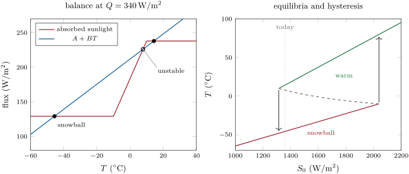
As $Q$ falls, the warm equilibrium cools and the ramp equilibrium warms. They meet at the top of the ramp, $T = T_F$, where $Q(1 - 0.30) = A + 10B$: $Q = 328.7\,\mathrm{W}/\mathrm{m}^{2}$, a solar constant of $1315\,\mathrm{W}/\mathrm{m}^{2}$, $3.3\,\%$ below today’s. That is a saddle-node bifurcation: below it the only equilibrium is the snowball, and the climate falls into it. Raising the Sun again does not bring the warm planet back: the snowball branch ends only where its temperature reaches $T_I$, $Q(1 - 0.62) = A - 10B$, at a solar constant of $2039\,\mathrm{W}/\mathrm{m}^{2}$, $50\,\%$ above today’s. Between the two, the state of the planet depends on its history: the model has hysteresis. In the real Neoproterozoic the way out of the snowball of the Year 2 volume was not a brighter Sun but the carbon dioxide of volcanoes, building up over millions of years until the greenhouse forcing reached the deglaciation threshold; the ice line then retreated to the poles in a few thousand years.

22.3 The Budyko–Sellers model

A single temperature has no ice line. In 1969 Budyko let the temperature depend on latitude and asked how far a reduction of the sunlight would push the ice towards the equator.

Definition 22.5 (Budyko–Sellers model)

A Budyko–Sellers model is an energy-balance model in which the annual mean temperature $T(x)$ depends on $x = \sin\varphi$, $\varphi$ the latitude, the hemispheres being symmetric. At each latitude

$$C\,\frac{\partial T}{\partial t} = Qs(x)\big(1 - \alpha(x)\big) - (A + BT) - D(x) ,$$

where $s(x)$ is the annual insolation of the latitude divided by its global mean, $D(x)$ the divergence of the poleward heat transport, and the albedo takes its ice value poleward of the ice line $x_s$, where $T$ falls below a critical temperature $T_c$. Budyko wrote $D = \beta(T - \bar T)$, a relaxation towards the global mean $\bar T$; in the diffusive form, $D = -\mathcal D\,\partial_x\big[(1 - x^2)\,\partial_xT\big]$.

The factor $x = \sin\varphi$ is chosen because equal intervals of $x$ hold equal areas of the sphere, so that a global mean is $\int_0^1\cdot\,\mathrm dx$. Budyko found $\beta = 0.235\,\mathrm{kcal}\,\mathrm{cm}^{-2}$ per month and per degree, $3.74\,\mathrm{W}\,\mathrm{m}^{-2}\,{}^{\circ}\mathrm{C}^{-1}$, from the observed distribution of temperature with latitude. He set the albedo to 0.62 on the ice and to 0.50 at its edge, where the ice is broken, and took the present ice edge at a mean latitude of $72{}^{\circ}$ N; the critical temperature is the one that puts the edge there.

Proposition 22.6 (The ice line of Budyko’s model)

Let $F(x_s) = \int_0^{x_s}s\,\mathrm dx$ be the fraction of the sunlight that falls equatorward of the ice line, and $\bar\alpha = \alpha_FF + \alpha_I(1 - F)$ the mean albedo weighted by sunlight. In a steady state of Budyko’s model,

$$B\bar T = Q(1 - \bar\alpha) - A, \qquad T(x) = \frac{Qs(x)\big(1 - \alpha(x)\big) - A + \beta\bar T}{B + \beta} ,$$

and an ice line at $x_s$, where $T = T_c$ with the edge albedo $\alpha_e$, needs

$$Q(x_s) = \frac{(B + \beta)T_c + A(1 + \beta/B)}{s(x_s)(1 - \alpha_e) + (\beta/B)\big(1 - \bar\alpha(x_s)\big)} .$$

An ice line is stable where $\mathrm dQ/\mathrm dx_s > 0$ and unstable where $\mathrm dQ/\mathrm dx_s < 0$.

Its meaning is the one of the zero-dimensional model: along a stable branch a little more sunshine pushes the ice line poleward. The temperature at which the edge sits today fixes $T_c = -12.3\,{}^{\circ}\mathrm{C}$; the reanalysis gives $-15.8\,{}^{\circ}\mathrm{C}$ at $72{}^{\circ}$, the mean of the two hemispheres. The model’s profile below is cooler than the observed one in the tropics and much warmer near the poles: a single coefficient $\beta$ cannot fit the whole profile. Its global mean, $12.8\,{}^{\circ}\mathrm{C}$, and its equator, $22.8\,{}^{\circ}\mathrm{C}$, are close to the observed $14.2\,{}^{\circ}\mathrm{C}$ and $25.7\,{}^{\circ}\mathrm{C}$.

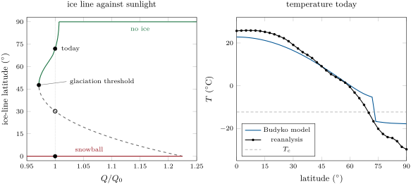
The stable branch has a minimum. With these values it lies at $47.7{}^{\circ}$, for $Q/Q_0 = 0.9713$: a fall of $2.87\,\%$ in the sunlight brings the ice to the middle latitudes, and any further fall sends it to the equator. Budyko found a smaller threshold with his own coefficients: a fall of $1.6\,\%$ brought his ice to a mean latitude of about $50{}^{\circ}$, after which it advanced to the equator of itself and the mean temperature fell to several tens of degrees below zero. The fit of the OLR and the albedos move the number; the shape of the curve, its minimum and the runaway beyond it do not. The diffusive form of the model, solved with Legendre polynomials in $x$, gives the same shape (exercise 22.10 treats a planet without ice).

22.4 Two-layer models

The response time of the one-box model, a few years, is that of the upper ocean. Below it the deep ocean takes up heat for centuries, and while it does the surface stays cooler than its equilibrium.

Definition 22.7 (Two-layer energy-balance model)

A two-layer energy-balance model represents the climate by a surface layer of temperature anomaly $T$ and heat capacity $C$, and a deep ocean of temperature anomaly $T_d$ and heat capacity $C_d$, coupled by a heat exchange coefficient $\gamma > 0$:

$$C\,\frac{\mathrm dT}{\mathrm dt} = F + \lambda T - \gamma(T - T_d), \qquad C_d\,\frac{\mathrm dT_d}{\mathrm dt} = \gamma(T - T_d) .$$

Theorem 22.8 (Fast and slow responses)

Let $\lambda < 0$, $\gamma > 0$, $C, C_d > 0$, and let a constant forcing $F$ start at $t = 0$ from equilibrium. Then

$$T(t) = -\frac{F}{\lambda}\Big(1 - a_f\,\mathrm e^{-t/\tau_f} - a_s\,\mathrm e^{-t/\tau_s}\Big), \qquad a_f + a_s = 1 ,$$

where $1/\tau_f$ and $1/\tau_s$ are the roots of $r^2 - \big((\gamma - \lambda)/C + \gamma/C_d\big)r - \lambda\gamma/(CC_d) = 0$. When $C \ll C_d$,

$$\tau_f \approx \frac{C}{\gamma - \lambda}, \qquad \tau_s \approx \frac{C_d(\gamma - \lambda)}{-\lambda\gamma}, \qquad a_f \approx \frac{-\lambda}{\gamma - \lambda} .$$

The emulator of the assessment, calibrated to 44 models, has $C = 8.1\,\mathrm{W}\,\mathrm{yr}\,\mathrm{m}^{-2}\,{}^{\circ}\mathrm{C}^{-1}$, $C_d = 110\,\mathrm{W}\,\mathrm{yr}\,\mathrm{m}^{-2}\,{}^{\circ}\mathrm{C}^{-1}$ and $\gamma = 0.62\,\mathrm{W}\,\mathrm{m}^{-2}\,{}^{\circ}\mathrm{C}^{-1}$; its feedback parameter is sampled about $\lambda = -1.33\,\mathrm{W}\,\mathrm{m}^{-2}\,{}^{\circ}\mathrm{C}^{-1}$. These values give $\tau_f = 4.1\text{ years}$ and $\tau_s = 262\text{ years}$, with $a_f = 0.67$: $62\,\%$ of the warming comes within a decade, most of the rest over centuries. The emulator also multiplies the heat exchange in the first equation by an efficacy $\varepsilon = 1.34$, which slows the surface further; it is set to 1 here.

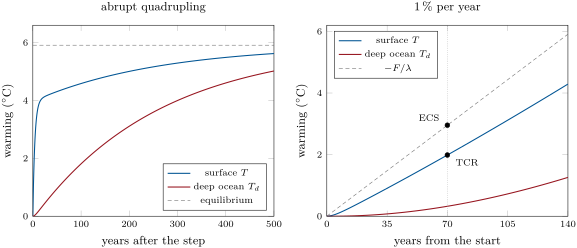
The model gives the two sensitivities of the Year 2 volume. Its ECS is $-F_{2\times}/\lambda = 3.93/1.33 = 2.95\,{}^{\circ}\mathrm{C}$. During a ramp lasting decades the deep ocean, with its time scale of centuries, has hardly warmed, and the surface is close to the fast balance $T \approx F/(\gamma - \lambda)$: the TCR is about $3.93/1.95 = 2.0\,{}^{\circ}\mathrm{C}$, against $1.99\,{}^{\circ}\mathrm{C}$ for the integration. With the efficacy, $\gamma$ is replaced by $\kappa = \varepsilon\gamma = 0.84\,\mathrm{W}\,\mathrm{m}^{-2}\,{}^{\circ}\mathrm{C}^{-1}$, and $\text{TCR} = F_{2\times}/(\kappa - \lambda) = 1.8\,{}^{\circ}\mathrm{C}$, the best estimate assessed by the report, which also assesses an ECS of $3\,{}^{\circ}\mathrm{C}$, likely 2.5 to $4\,{}^{\circ}\mathrm{C}$ (high confidence). The assessment finds that the differences of $\gamma$ and $\varepsilon$ between models explain 10 to $20\,\%$ of their spread of TCR.

A model this simple, tuned to reproduce the global temperature of a large model, is an emulator. The assessment ran a simple climate model whose temperature module is this two-layer model as an ensemble of a million members, sampled over the ranges of its parameters, and kept the 2237 members that reproduced the observed warming since 1850, the heat taken up by the ocean, the carbon dioxide of the air and the fraction of emissions that stays in it.

22.5 General circulation models

An energy-balance model is given its feedbacks and its transport; a general circulation model computes them from the laws of physics.

Definition 22.9 (General circulation model; dynamical core; parameterisation)

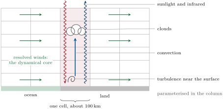
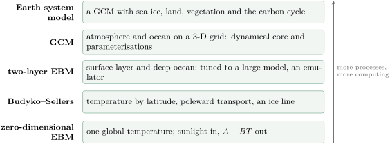
A general circulation model (GCM) is a numerical model of the atmosphere, of the ocean, or of both coupled, that solves the equations of motion, continuity and energy of a fluid on the rotating Earth — for the atmosphere, with the hydrostatic approximation, the “primitive equations” — on a three-dimensional grid covering the globe, stepping forward in time. Its dynamical core is the part that solves these equations for the motions the grid resolves. A parameterisation represents the effect on the resolved variables of a process smaller than a grid cell — clouds, convection, turbulence, gravity waves — by a formula in the resolved variables, with parameters that the modellers choose.

The resolution decides what must be parameterised. The general circulation models of 1990 had grid cells about $500\,\mathrm{km}$ across; the global models of the last assessment, about $100\,\mathrm{km}$; regional models, 25 to $50\,\mathrm{km}$, and a dedicated intercomparison has explored global grids of about 50, 25 and even $10\,\mathrm{km}$. A single convective cloud is much smaller than a global cell: convection is parameterised, and regional models fine enough to resolve it are now included in the intercomparisons.

Definition 22.10 (Earth system model)

An Earth system model (ESM) is a general circulation model of the atmosphere and the ocean coupled to models of the sea ice, the land surface and its vegetation, and of the carbon cycle, so that the concentrations of greenhouse gases and the properties of the surface can respond to the climate they help to set.

Earth system models are the most complex models used by the assessment. In the 1990s the coupled atmosphere–ocean models were the state of the art; by the 2010s land, vegetation and the carbon cycle had been added, and ice-sheet models are being coupled to them. Most of their projections are nevertheless run with prescribed concentrations of the greenhouse gases; only the emission-driven runs let the model’s carbon cycle compute them. Between the energy-balance models and the ESMs lies a hierarchy of models of intermediate complexity, cheap enough to be run for many thousands of years without a supercomputer.

Definition 22.11 (Spin-up)

The spin-up of a climate model is its integration under constant forcing, from an initial state, until its slow components — above all the deep ocean and the carbon stores — have stopped drifting; the experiments start from the state it reaches.

The two-layer model shows why a spin-up is long: its slow time scale is $262$ years, and after three of them, nearly eight centuries, the drift is still $5\,\%$ of the initial imbalance. The assessment notes that the different strategies used to spin up the models affected their performance.

22.6 Evaluating models

A model is tested against the observed climate; the trouble is that it has also been adjusted to it. Each parameterisation has parameters whose acceptable range is set by physics and observation, and as the components are assembled the modellers refine them until the simulated climate meets a set of tuning targets: the mean climate — for example, a mean temperature close to the observed one under today’s sunlight — regional features, or the trends of the historical period. Only then is the model released for the intercomparisons.

Definition 22.12 (Model intercomparison project)

A model intercomparison project is a coordinated set of experiments — the same forcings, the same protocols, the same outputs — run by many modelling groups with their own models, so that the results can be compared. The Coupled Model Intercomparison Project (CMIP) runs in successive phases; its sixth phase, CMIP6, was a key line of evidence of the sixth assessment.

Figures as of 2021

Of 29 modelling groups of CMIP6 that reported how they tuned, 23 did not tune their model to the warming observed during the historical period, and 25 did not tune its ECS: the sensitivity of most models is an emergent property, not an input. On average the CMIP6 models have a higher ECS and TCR than those of the previous phase, and a wider spread than the ranges assessed by the report; in some models this was traced to the feedback of the clouds of middle and high latitudes. Some of the most sensitive models reproduce the observed recent warming and the climates of the past less well. The assessment therefore did not take its ranges of ECS and TCR from the models directly, but from the understanding of the feedback processes, the instrumental record, the past climates and emergent constraints; it treats the most sensitive models as a guide to outcomes of low likelihood and high impact (high confidence).

Definition 22.13 (Large ensemble; emergent constraint)

A large ensemble is a set of many simulations by a single model, with the same forcings over the same period, that differ only in their initial states. An emergent constraint is a relationship, found across an ensemble of different models, between an observable quantity of the present climate and a quantity of the future one, such as the ECS; the observed value of the first then narrows the range of the second.

The climate is chaotic, so tiny differences of the initial state send the members of a large ensemble along different paths: the spread of the members measures the internal variability, and their mean the forced response. Large ensembles of several models supported the assessment. An emergent constraint needs a physical reason. Across a few dozen models, thousands of observables can be tried, and some will correlate with the ECS by chance; the assessment kept those with a physical basis, many of them about the clouds of the tropics, and warned that a bias shared by all the models of the ensemble defeats the method.

In the lab — A modelling centre

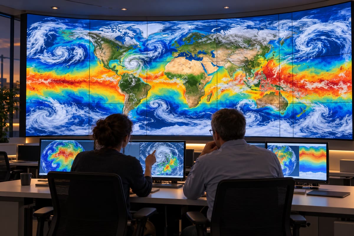
At a climate modelling centre, the model is a program written and maintained by a team: atmosphere, ocean, sea ice and land are separate components, exchanging fluxes at their interfaces through a coupler. Before a run, the experiment’s forcings are read in — the concentrations of greenhouse gases, the aerosols, the land use of the protocol. The globe is cut into pieces that the processors of the supercomputer compute side by side, and a century of model climate comes back as a large archive of fields. The scientists display them on screens, compare them with reanalyses and satellite records, and send the standard outputs to the intercomparison’s archive, where other groups compare them with their own.

22.7 Exercises

Exercise 22.1 ★

Budyko’s OLR law is $I = a + bT - (a_1 + b_1T)n$, with $a = 14.0$, $b = 0.14$, $a_1 = 3.0$, $b_1 = 0.10$, in $\mathrm{kcal}\,\mathrm{cm}^{-2}$ per month and $T$ in ${}^{\circ}\mathrm{C}$. For a cloudiness $n = 0.5$, compute $A$ and $B$, and convert them to $\mathrm{W}/\mathrm{m}^{2}$ and $\mathrm{W}\,\mathrm{m}^{-2}\,{}^{\circ}\mathrm{C}^{-1}$, with a month a twelfth of a year of 365.25 days. What OLR does the law give at $15\,{}^{\circ}\mathrm{C}$?

Solution

Solution of Exercise 22.1.

$A = 14.0 - 1.5 = 12.5$ and $B = 0.14 - 0.05 = 0.09$, in $\mathrm{kcal}\,\mathrm{cm}^{-2}$ per month. A month is $2.63 \times 10^{6}\,\mathrm{s}$, so $1\,\mathrm{kcal}\,\mathrm{cm}^{-2}$ per month is $4.184 \times 10^{7}/2.63 \times 10^{6} = 15.91\,\mathrm{W}/\mathrm{m}^{2}$: $A = 199\,\mathrm{W}/\mathrm{m}^{2}$, $B = 1.43\,\mathrm{W}\,\mathrm{m}^{-2}\,{}^{\circ}\mathrm{C}^{-1}$. At $15\,{}^{\circ}\mathrm{C}$, $199 + 21.5 = 220\,\mathrm{W}/\mathrm{m}^{2}$.

Exercise 22.2 ★

With $Q = 340\,\mathrm{W}/\mathrm{m}^{2}$, $A = 211.9\,\mathrm{W}/\mathrm{m}^{2}$ and $B = 1.816\,\mathrm{W}\,\mathrm{m}^{-2}\,{}^{\circ}\mathrm{C}^{-1}$, compute the equilibrium temperature for an albedo of 0.30 and of 0.31. By how much does a rise of 0.01 of the albedo cool this planet?

Solution

Solution of Exercise 22.2.

$(238.0 - 211.9)/1.816 = 14.4\,{}^{\circ}\mathrm{C}$; with 0.31, $(234.6 - 211.9)/1.816 = 12.5\,{}^{\circ}\mathrm{C}$. Each 0.01 of albedo costs $3.4\,\mathrm{W}/\mathrm{m}^{2}$ and $3.4/1.816 = 1.9\,{}^{\circ}\mathrm{C}$.

Exercise 22.3 ★

Compute the heat capacity per square metre of a mixed layer of sea water $60\,\mathrm{m}$ deep, $\rho = 1025\,\mathrm{kg}/\mathrm{m}^{3}$ and $c_p = 3992\,\mathrm{J}\,\mathrm{kg}^{-1}\,\mathrm{K}^{-1}$, in $\mathrm{J}\,\mathrm{m}^{-2}\,\mathrm{K}^{-1}$ and in $\mathrm{W}\,\mathrm{yr}\,\mathrm{m}^{-2}\,\mathrm{K}^{-1}$. Compute the response time of Theorem 22.2 for $\lambda = -B = -1.816\,\mathrm{W}\,\mathrm{m}^{-2}\,{}^{\circ}\mathrm{C}^{-1}$ and for $\lambda = -1.33\,\mathrm{W}\,\mathrm{m}^{-2}\,{}^{\circ}\mathrm{C}^{-1}$.

Solution

Solution of Exercise 22.3.

$C = 1025\times3992\times60 = 2.46 \times 10^{8}\,\mathrm{J}\,\mathrm{m}^{-2}\,\mathrm{K}^{-1}$; divided by the $3.156 \times 10^{7}\,\mathrm{s}$ of a year, $7.78\,\mathrm{W}\,\mathrm{yr}\,\mathrm{m}^{-2}\,\mathrm{K}^{-1}$. Then $\tau = 7.78/1.816 = 4.3\text{ years}$, and $7.78/1.33 = 5.8\text{ years}$.

Exercise 22.4 ★

For the two-layer model with $\lambda = -1.33\,\mathrm{W}\,\mathrm{m}^{-2}\,{}^{\circ}\mathrm{C}^{-1}$, $\gamma = 0.62\,\mathrm{W}\,\mathrm{m}^{-2}\,{}^{\circ}\mathrm{C}^{-1}$ and $F_{2\times} = 3.93\,\mathrm{W}/\mathrm{m}^{2}$, compute the ECS, the approximate TCR $F_{2\times}/ (\gamma - \lambda)$, and their ratio.

Solution

Solution of Exercise 22.4.

ECS $= 3.93/1.33 = 2.95\,{}^{\circ}\mathrm{C}$; TCR $\approx 3.93/1.95 = 2.02\,{}^{\circ}\mathrm{C}$; ratio $0.68$.

Exercise 22.5 ★★

In the zero-dimensional model of the text, take a solar constant of $1340\,\mathrm{W}/\mathrm{m}^{2}$. Find the three equilibria and the slope $N'(T)$ of the net flux at each; which are stable?

Solution

Solution of Exercise 22.5.

$Q = 335\,\mathrm{W}/\mathrm{m}^{2}$. Snowball: $(335\times0.38 - 211.9)/1.816 = -46.6\,{}^{\circ}\mathrm{C}$; warm: $(335\times0.70 - 211.9)/1.816 = 12.4\,{}^{\circ}\mathrm{C}$, still above $10\,{}^{\circ}\mathrm{C}$; ramp: $335(0.54 + 0.016\,T) = 211.9 + 1.816\,T$ gives $T = 8.7\,{}^{\circ}\mathrm{C}$. $N' = -1.816\,\mathrm{W}\,\mathrm{m}^{-2}\,{}^{\circ}\mathrm{C}^{-1}$ at the first two, stable, and $-1.816 + 335\times0.016 = +3.54$ at the ramp, unstable.

Exercise 22.6 ★★

Move the albedo ramp of the text: $\alpha = 0.62$ below $-20\,{}^{\circ}\mathrm{C}$, $0.30$ above $0\,{}^{\circ}\mathrm{C}$, linear between. Keep $A$ and $B$. At what solar constant does the warm branch end, and by how many per cent is that below $1360\,\mathrm{W}/\mathrm{m}^{2}$? At what solar constant does the snowball melt? What sets the size of the threshold?

Solution

Solution of Exercise 22.6.

The warm branch ends where its temperature reaches $0\,{}^{\circ}\mathrm{C}$: $0.70\,Q = A$, $Q = 302.7\,\mathrm{W}/\mathrm{m}^{2}$, a solar constant of $1211\,\mathrm{W}/\mathrm{m}^{2}$, $11.0\,\%$ below today’s. The snowball melts where $0.38\,Q = A - 20B$, $Q = 462.1\,\mathrm{W}/\mathrm{m}^{2}$, $S_0 = 1848\,\mathrm{W}/\mathrm{m}^{2}$. The threshold is $B(T^* - T_F)/(Q_0(1 - \alpha_F))$, the gap between today’s temperature $T^*$ and the temperature at which the ice starts to spread, converted to sunlight: $1.816\times14.37/238 = 11.0\,\%$ here, $1.816\times4.37/238 = 3.3\,\%$ in the text.

Exercise 22.7 ★★

A model planet with the parameters of the text is in the snowball state. (a) What is its temperature at today’s solar constant? (b) Keeping the Sun as it is, what forcing $F$ would bring the snowball’s temperature up to $-10\,{}^{\circ}\mathrm{C}$? How many times the forcing of a doubling of carbon dioxide, $3.93\,\mathrm{W}/\mathrm{m}^{2}$, is it? (c) Once the ice has gone, where does the planet settle if the forcing is then removed?

Solution

Solution of Exercise 22.7.

(a) $-45.5\,{}^{\circ}\mathrm{C}$. (b) $340\times0.38 + F = 211.9 - 18.2$: $F = 64.5\,\mathrm{W}/\mathrm{m}^{2}$, 16 times the forcing of a doubling. (c) While the forcing lasts the planet jumps to the warm branch, $(238.0 + 64.5 - 211.9)/1.816 = 50\,{}^{\circ}\mathrm{C}$; once it is removed the planet cools along the warm branch to $14.4\,{}^{\circ}\mathrm{C}$, which exists at today’s Sun: it does not return to the snowball.

Exercise 22.8 ★★

Model X, an invented two-layer model, has $C = 7.0$ and $C_d = 90\,\mathrm{W}\,\mathrm{yr}\,\mathrm{m}^{-2}\,{}^{\circ}\mathrm{C}^{-1}$, $\gamma = 0.70$ and $\lambda = -1.10\,\mathrm{W}\,\mathrm{m}^{-2}\,{}^{\circ}\mathrm{C}^{-1}$. Compute its two time scales exactly and with the approximations of Theorem 22.8, the fraction $a_f$, its ECS and its approximate TCR.

Solution

Solution of Exercise 22.8.

$\Sigma = 1.80/7.0 + 0.70/90 = 0.2649\,\mathrm{yr}^{-1}$, $\Pi = 1.10\times0.70/ (7.0\times90) = 1.222 \times 10^{-3}\,\mathrm{yr}^{-2}$. The roots give $\tau_f = 3.84\text{ years}$ and $\tau_s = 213\text{ years}$; the approximations, $7.0/1.80 = 3.89\text{ years}$ and $90\times1.80/(1.10\times0.70) = 210\text{ years}$. $a_f = 0.597$ exactly, $1.10/1.80 = 0.611$ approximately. ECS $= 3.93/1.10 = 3.57\,{}^{\circ}\mathrm{C}$; TCR $\approx 3.93/1.80 = 2.18\,{}^{\circ}\mathrm{C}$.

Exercise 22.9 ★★

In Budyko’s model of the text, $\bar T = 12.81\,{}^{\circ}\mathrm{C}$, $\beta = 3.74\,\mathrm{W}\,\mathrm{m}^{-2}\,{}^{\circ}\mathrm{C}^{-1}$, the ice line at $72{}^{\circ}$, $s = 1.221$ at the equator and $0.506$ at the pole, $\alpha = 0.30$ and $0.62$. Compute the temperature at the equator and at the pole, and the heat $\beta(T - \bar T)$ that the transport removes from, or brings to, each square metre there.

Solution

Solution of Exercise 22.9.

Denominator $B + \beta = 5.555$. Equator: $(340\times1.221\times0.70 - 211.9 + 3.74\times12.81)/5.555 = 22.8\,{}^{\circ}\mathrm{C}$; pole: $(340\times0.506\times0.38 - 211.9 + 47.9)/5.555 = -17.7\,{}^{\circ}\mathrm{C}$. The transport removes $3.74\times(22.8 - 12.8) = 37\,\mathrm{W}/\mathrm{m}^{2}$ at the equator and brings $3.74\times30.6 = 114\,\mathrm{W}/\mathrm{m}^{2}$ to the pole.

Exercise 22.10 ★★★

A planet without ice ($\alpha = 0.30$ everywhere) has the diffusive transport $D = -\mathcal D\,\partial_x[(1 - x^2)\partial_xT]$ and the insolation $s(x) = 1 + s_2P_2(x)$, $P_2 = (3x^2 - 1)/2$. (a) Show that $\partial_x[(1 - x^2)\partial_xP_2] = -6P_2$. (b) Show that $T = T_0 + T_2P_2(x)$ is a steady solution, with $T_0 = (Q(1 - \alpha) - A)/B$ and $T_2 = Qs_2(1 - \alpha)/(B + 6\mathcal D)$. (c) The insolation of the reanalysis gives $s_2 = -0.476$. Without transport, what would be the temperature difference between equator and pole? (d) What $\mathcal D$ gives the observed difference, $55.3\,{}^{\circ}\mathrm{C}$?

Solution

Solution of Exercise 22.10.

(a) $(1 - x^2)P_2' = 3x - 3x^3$, whose derivative is $3 - 9x^2 = -6P_2$. (b) The transport term is $-\mathcal D T_2(-6P_2) = 6\mathcal DT_2P_2$. The balance $Q(1 + s_2P_2)(1 - \alpha) - A - B(T_0 + T_2P_2) - 6\mathcal DT_2P_2 = 0$ holds for all $x$ if its constant part and its $P_2$ part vanish, which gives $T_0$ and $T_2$. (c) $T(0) - T(1) = T_2(-\tfrac12 - 1) = -1.5\,T_2$. Without transport $T_2 = 340\times(-0.476)\times0.70/1.816 = -62.4\,{}^{\circ}\mathrm{C}$: a difference of $94\,{}^{\circ}\mathrm{C}$. (d) $T_2 = -55.3/1.5 = -36.9\,{}^{\circ}\mathrm{C}$, so $B + 6\mathcal D = 113.3/36.9 = 3.07$ and $\mathcal D = 0.21\,\mathrm{W}\,\mathrm{m}^{-2}\,{}^{\circ}\mathrm{C}^{-1}$.

Exercise 22.11 ★★★

(a) Write the quadratic of Theorem 22.8 as $r^2 - \Sigma r + \Pi = 0$ and show that, if $4\Pi \ll \Sigma^2$, its roots are close to $\Sigma$ and $\Pi/\Sigma$. (b) For a forcing $F = kt$ rising linearly, show that once $t \gg \tau_f$, and while $T_d$ stays small, $T \approx kt/(\gamma - \lambda)$; deduce the approximate TCR. (c) Check the numbers of the text: $\Sigma$, $\Pi$, the two time scales, and the ratio $4\Pi/\Sigma^2$.

Solution

Solution of Exercise 22.11.

(a) $r = \tfrac12\Sigma\big(1 \pm \sqrt{1 - 4\Pi/\Sigma^2}\big)$; with $\sqrt{1 - \epsilon} \approx 1 - \epsilon/2$, the roots are $\Sigma - \Pi/\Sigma \approx \Sigma$ and $\Pi/\Sigma$. (b) With $T_d = 0$, $C\,\mathrm dT/\mathrm dt = kt - (\gamma - \lambda)T$, whose solution from rest is $T = k(t - \tau_f)/(\gamma - \lambda) + k\tau_f\mathrm e^{-t/\tau_f}/(\gamma - \lambda)$, $\tau_f = C/(\gamma - \lambda)$. For $t \gg \tau_f$, $T \approx kt/(\gamma - \lambda)$, and at the doubling, $kt = F_{2\times}$: TCR $\approx F_{2\times}/(\gamma - \lambda)$. (c) $\Sigma = 1.95/8.1 + 0.62/110 = 0.2464\,\mathrm{yr}^{-1}$, $\Pi = 1.33\times0.62/(8.1\times110) = 9.25 \times 10^{-4}\,\mathrm{yr}^{-2}$; $\tau_f = 4.12\text{ years}$ and $\tau_s = 262\text{ years}$ (approximately $1/\Sigma = 4.06\text{ years}$ and $\Sigma/\Pi = 266\text{ years}$); $4\Pi/\Sigma^2 = 0.061$.

Exercise 22.12 ★★★

An invented ensemble of eight models gives an observable $X$ of the present climate and their ECS:

$X$	0.2	0.5	0.6	0.8	1.0	1.1	1.3	1.5
ECS (${}^{\circ}\mathrm{C}$)	2.3	2.7	3.1	3.2	3.8	3.9	4.4	4.6

(a) Compute the mean and the standard deviation of the ECS of the ensemble. (b) Fit ECS $= a + bX$ by least squares; compute the correlation and the standard deviation of the residuals. (c) The observed $X$ is $0.7 \pm 0.1$. What ECS does the constraint give, and with what spread? (d) What would make you distrust this constraint?

Solution

Solution of Exercise 22.12.

(a) Mean $3.50\,{}^{\circ}\mathrm{C}$, standard deviation $0.81\,{}^{\circ}\mathrm{C}$. (b) ECS $= 1.88 + 1.86\,X$; correlation $0.992$; residual standard deviation $0.11\,{}^{\circ}\mathrm{C}$. (c) $1.88 + 1.86\times0.7 = 3.18\,{}^{\circ}\mathrm{C}$, with a spread $\sqrt{(1.86\times0.1)^2 + 0.11^2} = 0.22\,{}^{\circ}\mathrm{C}$, about a quarter of the spread of the ensemble. (d) No physical mechanism linking $X$ to the feedbacks; an $X$ found by trying many observables, so that the correlation may be chance; a bias shared by all eight models; models of the same family counted as independent.

22.8 Problem: How Close to a Snowball?

Problem 22.1

Weekend problem — equilibria, stability and the glaciation threshold of a model planet

A model planet has today’s solar constant $S_0 = 1360\,\mathrm{W}/\mathrm{m}^{2}$ and the OLR law $A + BT$ with $A = 211.9\,\mathrm{W}/\mathrm{m}^{2}$ and $B = 1.816\,\mathrm{W}\,\mathrm{m}^{-2}\,{}^{\circ}\mathrm{C}^{-1}$. Its albedo is 0.62 below $-10\,{}^{\circ}\mathrm{C}$, 0.30 above $+10\,{}^{\circ}\mathrm{C}$, linear between, and its surface heat capacity $C = 8.1\,\mathrm{W}\,\mathrm{yr}\,\mathrm{m}^{-2}\,{}^{\circ}\mathrm{C}^{-1}$. Take $\sigma = 5.670 \times 10^{-8}\,\mathrm{W}\,\mathrm{m}^{-2}\,\mathrm{K}^{-4}$.

Part I — The planet in balance.

1. Compute the mean sunlight $Q_0$ per square metre of the planet, and explain the factor.
2. Compute the absorbed sunlight with an albedo of 0.30, and the OLR at $15\,{}^{\circ}\mathrm{C}$.
3. Compute the warm equilibrium.
4. Compute the snowball equilibrium, and check that it lies on the icy branch.
5. Compute the third equilibrium, on the albedo ramp.
6. Compute the emission temperature that sends the absorbed sunlight back to space as a black body, and compare it with the warm equilibrium.

Part II — Stability and time.

7. Compute the slope $N'(T)$ of the net flux at each equilibrium, and say which are stable.
8. A small departure from the middle equilibrium grows as $\mathrm e^{t/\tau}$. Compute $\tau$.
9. Compute the response time of the warm equilibrium.
10. A forcing of $3.93\,\mathrm{W}/\mathrm{m}^{2}$, that of a doubling of carbon dioxide, is switched on. Compute the warming at equilibrium, and compare it with the ECS assessed for the real climate.
11. How long does the model take to cover $95\,\%$ of the warming? Why does the real climate take longer?

Part III — The saddle-node.

12. As the Sun dims, at what temperature does the warm equilibrium meet the middle one? Compute $Q$ there.
13. Compute the solar constant at the bifurcation, and the drop from today in per cent.
14. Just below it, where does the climate go? Compute its temperature.
15. Compute the solar constant at which the snowball melts, and the rise from today in per cent.
16. Sketch the loop followed by the temperature when $S_0$ is lowered below the bifurcation and brought back to $1360\,\mathrm{W}/\mathrm{m}^{2}$.

Part IV — The ice line. Give the planet Budyko’s latitudinal model, with $\beta = 3.739\,\mathrm{W}\,\mathrm{m}^{-2}\,{}^{\circ}\mathrm{C}^{-1}$, an ice albedo of 0.62 poleward of the ice line, 0.30 equatorward, 0.50 at the edge, and the insolation of the reanalysis:

latitude	$0{}^{\circ}$	$30{}^{\circ}$	$40{}^{\circ}$	$47.5{}^{\circ}$	$55{}^{\circ}$	$60{}^{\circ}$	$72{}^{\circ}$
$s(x_s)$	1.2211	1.0730	0.9647	0.8688	0.7650	0.6947	0.5643
$F(x_s)$	0	0.5865	0.7324	0.8192	0.8863	0.9205	0.9738

17. With the ice line at $72{}^{\circ}$, compute the mean albedo $\bar\alpha$ and the mean temperature $\bar T$.
18. Compute the critical temperature $T_c$ that puts the edge at $72{}^{\circ}$ today, and compare it with the reanalysis, $-15.8\,{}^{\circ}\mathrm{C}$.
19. Compute the numerator of $Q(x_s)$ in Proposition 22.6 and the ratio $\beta/B$.
20. Compute $Q(x_s)/Q_0$ for the ice line at $30{}^{\circ}$, $40{}^{\circ}$, $47.5{}^{\circ}$, $55{}^{\circ}$ and $60{}^{\circ}$.
21. Where is the minimum of these values? Which ice lines are stable?
22. With today’s Sun, what other ice line does the model allow, and is it stable? Is the snowball possible today? (Use the column $0{}^{\circ}$.)
23. Compare the threshold of the latitudinal model with that of Part III and with Budyko’s $1.6\,\%$, and the latitude of the ice at the threshold with his $50{}^{\circ}$.
24. Give, to two significant figures, the fall of the solar constant, in per cent, that glaciates the model planet.

Solution

Solution of Problem 22.1.

1. $Q_0 = 1360/4 = 340\,\mathrm{W}/\mathrm{m}^{2}$: the planet intercepts the sunlight on a disc of area $\pi R^2$ and spreads it over a sphere of area $4\pi R^2$.

2. $340\times0.70 = 238.0\,\mathrm{W}/\mathrm{m}^{2}$; $211.9 + 1.816\times15 = 239.1\,\mathrm{W}/\mathrm{m}^{2}$.

3. $(238.0 - 211.9)/1.816 = 14.4\,{}^{\circ}\mathrm{C}$.

4. $(129.2 - 211.9)/1.816 = -45.5\,{}^{\circ}\mathrm{C}$, below $-10\,{}^{\circ}\mathrm{C}$.

5. $340(0.54 + 0.016\,T) = 211.9 + 1.816\,T$: $T = (183.6 - 211.9)/(1.816 - 5.44) = 7.8\,{}^{\circ}\mathrm{C}$.

6. $(238.0/5.670 \times 10^{-8})^{1/4} = 254.5\,\mathrm{K}$, $-18.6\,{}^{\circ}\mathrm{C}$: $33\,{}^{\circ}\mathrm{C}$ below the warm equilibrium, the greenhouse effect of the planet built into $A$ and $B$.

7. $N' = -B = -1.816\,\mathrm{W}\,\mathrm{m}^{-2}\,{}^{\circ}\mathrm{C}^{-1}$ at the snowball and the warm equilibrium, both stable; $-1.816 + 5.44 = +3.62$ at the middle one, unstable.

8. $\tau = 8.1/3.62 = 2.2\text{ years}$.

9. $8.1/1.816 = 4.5\text{ years}$.

10. $3.93/1.816 = 2.2\,{}^{\circ}\mathrm{C}$, below the assessed best estimate of $3\,{}^{\circ}\mathrm{C}$ and below its likely range, 2.5 to $4\,{}^{\circ}\mathrm{C}$: the $B$ of the model, fitted across latitudes, is not the feedback parameter of the climate as a whole.

11. $\mathrm e^{-t/\tau} = 0.05$ at $t = 3\tau = 13\text{ years}$. The real climate also warms the deep ocean, whose time scale is centuries.

12. At $T_F = 10\,{}^{\circ}\mathrm{C}$; $Q = (211.9 + 18.2)/0.70 = 328.7\,\mathrm{W}/\mathrm{m}^{2}$.

13. $S_0 = 1315\,\mathrm{W}/\mathrm{m}^{2}$, $3.3\,\%$ below today’s.

14. To the snowball, $(328.7\times0.38 - 211.9)/1.816 = -47.9\,{}^{\circ}\mathrm{C}$.

15. $Q = (211.9 - 18.2)/0.38 = 509.8\,\mathrm{W}/\mathrm{m}^{2}$, $S_0 = 2039\,\mathrm{W}/\mathrm{m}^{2}$, $50\,\%$ above today’s.

16. Down the warm branch to $10\,{}^{\circ}\mathrm{C}$ at $1315\,\mathrm{W}/\mathrm{m}^{2}$, a fall to $-48\,{}^{\circ}\mathrm{C}$, then back up the snowball branch to $-45.5\,{}^{\circ}\mathrm{C}$ at $1360\,\mathrm{W}/\mathrm{m}^{2}$: the planet stays frozen. Only beyond $2039\,\mathrm{W}/\mathrm{m}^{2}$ would it jump back to the warm branch.

17. $\bar\alpha = 0.30\times0.9738 + 0.62\times0.0262 = 0.3084$; $\bar T = (340\times0.6916 - 211.9)/1.816 = 12.80\,{}^{\circ}\mathrm{C}$.

18. $T_c = (340\times0.5643\times0.50 - 211.9 + 3.739\times12.80)/ 5.555 = -12.26\,{}^{\circ}\mathrm{C}$, $3.5\,{}^{\circ}\mathrm{C}$ warmer than the reanalysis at $72{}^{\circ}$.

19. $5.555\times(-12.26) + 211.9\times3.059 = 580.1$, with $\beta/B = 2.059$.

20. The denominators are 1.7053, 1.7473, 1.7565, 1.7488 and 1.7362, and $Q/Q_0 = 1.0005$, $0.9764$, $0.9713$, $0.9756$ and $0.9827$.

21. Near $47.5{}^{\circ}$, at $0.971$. The ice lines poleward of the minimum are stable, $\mathrm dQ/\mathrm dx_s > 0$; those equatorward are unstable.

22. $Q/Q_0 = 1$ also between $30{}^{\circ}$ and $40{}^{\circ}$, close to $30{}^{\circ}$ ($30.2{}^{\circ}$ by interpolation): an unstable ice line. At $0{}^{\circ}$, $Q/Q_0 = 580.1/(0.6106 + 0.7824)/340 = 1.225$: the snowball holds for any Sun up to $22\,\%$ brighter than today’s, so it is possible today.

23. $2.9\,\%$, against $3.3\,\%$ for the zero-dimensional model and $1.6\,\%$ for Budyko; the ice stands near $48{}^{\circ}$ at the threshold, against his $50{}^{\circ}$. The latitudinal model glaciates sooner than the global one, because the sunlight is weakest where the ice forms.

24. The model planet glaciates for a fall of $2.9\,\%$ of the solar constant ($2.87\,\%$ by the calculation).