4Geomagnetism and Palaeomagnetism

A basalt flow erupted sixty million years ago cooled with its tiny grains of magnetite locked parallel to the field of the day. Drilled today, oriented in place, sliced into small cylinders and heated step by step in a room shielded from the present field, it still says how far it then lay from the pole and which way it faced. Thousands of such measurements, from every continent and every age, have told how the continents moved before the ocean floors that record their motion were born, and in which order the field has reversed through the layers of a sedimentary section. This chapter describes the field as it is today, how rocks record it, how a direction is extracted and averaged, and what a palaeomagnetic pole says about the motion of a plate.

You already know

The Earth as a magnet and the magnetic declination are in the physics books’ school volumes; magnetic domains, hysteresis, remanence and the Curie temperature in their Year 3 volume; the field of a magnetic dipole in their Year 1 volume. Magnetic reversals and the normal and reversed polarities were met in grade 11. The great circle and the spherical triangle were defined in the Year 1 volume, in its chapter on spherical astronomy; the polarity chron, the geomagnetic polarity timescale, the marine magnetic anomaly and finite rotations about an Euler pole in its chapter on plate kinematics on a sphere; the hotspot track in its chapter on hotspots. Spherical harmonics and the Schmidt-normalised Legendre functions $P_n^m$ were used for gravity in the chapter on gravity and the figure of the Earth (Chapter 3).

4.1 The main field

Definition 4.1 (Main geomagnetic field; geocentric axial dipole)

The main geomagnetic field is the part of the Earth’s magnetic field produced inside the Earth, in its liquid iron outer core; it changes over years to millions of years, unlike the fields of the ionosphere and the magnetosphere, which change over seconds to days. The geocentric axial dipole is the field of a magnetic dipole placed at the centre of the Earth and aligned with its rotation axis, pointing south, so that its field lines leave the southern hemisphere and enter the northern one.

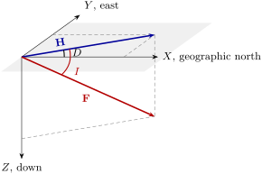
At any point of the surface the field $\mathbf F$ is a vector. It is described in a local frame (figure below): $X$ towards geographic north, $Y$ towards the east, $Z$ downwards. Its horizontal component is $H = \sqrt{X^2 + Y^2}$, its total intensity $F = |\mathbf F|$, its magnetic declination $D$ the angle from geographic north to $\mathbf H$, counted clockwise, and its inclination $I$ the angle from the horizontal to $\mathbf F$.

Definition 4.2 (Magnetic inclination)

The magnetic inclination $I$ of the field at a point is the angle between the field vector and the horizontal plane, positive when the field points downwards: $\tan I = Z/H$, with $-90{}^{\circ} \le I \le 90{}^{\circ}$.

Theorem 4.3 (The dipole formula)

At the surface of a sphere of radius $a$, the field of a geocentric axial dipole of moment $m$ has, at latitude $\lambda$,

$$H = B_0\cos\lambda,\qquad Z = 2B_0\sin\lambda,\qquad F = B_0\sqrt{1 + 3\sin^2\lambda},\qquad \tan I = 2\tan\lambda,\qquad D = 0,$$

where $B_0 = \mu_0 m/(4\pi a^3)$ is the field at the equator. This is the dipole formula.

The inclination is zero at the equator, $90{}^{\circ}$ at the north pole, and negative in the southern hemisphere; the intensity is twice as large at the poles as at the equator. The real field is not a perfect dipole, and it is described, like gravity, by spherical harmonics.

Definition 4.4 (International Geomagnetic Reference Field)

The International Geomagnetic Reference Field (IGRF) is the internationally agreed model of the main field: the potential, on and above the surface,

$$V(r,\theta,\varphi) = a\sum_{n=1}^{N}\Bigl(\frac ar\Bigr)^{n+1}\sum_{m=0}^{n} \bigl(g_n^m\cos m\varphi + h_n^m\sin m\varphi\bigr)P_n^m(\cos\theta),$$

with $a = 6371.2\,\mathrm{km}$, $\mathbf B = -\nabla V$, and Gauss coefficients $g_n^m$, $h_n^m$ (in $\mathrm{nT}$) given every five years since 1900, together with their rate of change over the next five years.

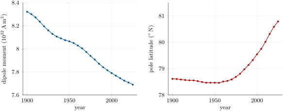
The model is maintained by the International Association of Geomagnetism and Aeronomy; its fourteenth generation was completed in November 2024 and is truncated at degree $N = 13$. The first term, $g_1^0$, is the axial dipole: comparing with the proof above, $B_0 = -g_1^0$, and $g_1^0 = -29\,350\,\mathrm{nT}$ in 2025. With the two other degree-1 terms the dipole is tilted; its axis meets the surface at the north geomagnetic pole, at $80.79{}^{\circ}$ N, $72.76{}^{\circ}$ W in 2025, and its moment is $m = 4\pi a^3\sqrt{(g_1^0)^2 + (g_1^1)^2 + (h_1^1)^2}/\mu_0 = 7.69 \times 10^{22}\,\mathrm{A}\,\mathrm{m}^{2}$.

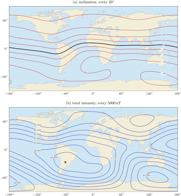
The maps above show how far the field departs from a dipole. The dip equator wanders up to about $12{}^{\circ}$ from the geographic equator, and the intensity, which a dipole would make uniform along a parallel, varies by a factor of three, with a broad low over the South Atlantic.

Definition 4.5 (Secular variation)

The secular variation is the slow change of the main field with time, over years to centuries, measured by the rate of change of its Gauss coefficients or of its elements at a place.

Over the last 125 years the dipole moment has fallen from $8.32 \times 10^{22}\,\mathrm{A}\,\mathrm{m}^{2}$ to $7.69 \times 10^{22}\,\mathrm{A}\,\mathrm{m}^{2}$, by $7.6\,\%$, and the north geomagnetic pole has moved from $78.61{}^{\circ}$ N, $68.79{}^{\circ}$ W to its present position (figure below); $g_1^0$ still grows by $12.6\,\mathrm{nT}$ a year, a weakening of the dipole.

Where does the field come from? A permanent magnet is ruled out: the Curie temperature of magnetite is about $580\,{}^{\circ}\mathrm{C}$ and that of haematite $675\,{}^{\circ}\mathrm{C}$, and the deep Earth is far hotter. The field is regenerated continuously by the motion of the conducting liquid of the outer core.

Definition 4.6 (Geodynamo)

The geodynamo is the self-sustaining process by which convection of the electrically conducting liquid iron alloy of the outer core, deflected by the Earth’s rotation, induces electric currents whose magnetic field maintains itself against ohmic decay.

Proposition 4.7 (Induction equation)

In a conductor of magnetic diffusivity $\eta = 1/(\mu_0\sigma)$ moving with the velocity $\mathbf u$, the magnetic field obeys

$$\frac{\partial\mathbf B}{\partial t} = \nabla\times(\mathbf u\times\mathbf B) + \eta\nabla^2\mathbf B .$$

The first term stretches and twists the field lines carried by the flow; the second makes the field decay, in a body of size $L$, in a time of order $L^2/\eta$. A dynamo works when the flow regenerates field faster than it diffuses away. Computer simulations of a convecting, rotating shell of fluid reproduce a dominant axial dipole and, now and then, a reversal; but the equations of the geodynamo, coupled with those of the flow, are beyond this book. Besides the full reversals, the record holds shorter events.

Definition 4.8 (Geomagnetic excursion)

A geomagnetic excursion is a large departure of the field direction from that of the axial dipole, the virtual geomagnetic pole (Definition 4.16) moving far from the geographic pole, which returns to the original polarity instead of completing a reversal.

4.2 How rocks record the field

Ferromagnetic minerals in the broad sense, chiefly magnetite in igneous rocks and haematite in red sediments, carry a remanence. Above its Curie temperature a grain has none; below it, a small grain is a single magnetic domain whose moment flips between its easy directions, thermally activated, after a relaxation time

where $K$ is the anisotropy energy per unit volume, $V$ the volume of the grain and $C$ a frequency factor. This is Néel’s relaxation law, admitted here. Since $\tau$ grows exponentially as $T$ falls, a grain passes over a narrow interval of temperature from flipping freely to holding its moment for billions of years.

Definition 4.9 (Blocking temperature)

The blocking temperature of a magnetic grain is the temperature below which its relaxation time exceeds the time of the experiment, so that its moment stays fixed: on cooling through it, the grain records the field; on heating through it in zero field, the grain loses that record.

Definition 4.10 (Natural, thermal, detrital and chemical remanent magnetisation)

The natural remanent magnetisation (NRM) of a rock is the remanence it carries as it is collected, the sum of components acquired at different times. A thermoremanent magnetisation (TRM) is acquired by cooling through the blocking temperatures in a field, as in a lava flow or an intrusion. A detrital remanent magnetisation (DRM) is acquired when magnetic grains settling in water, or in the wet sediment just below its surface, rotate into the field before they are locked. A chemical remanent magnetisation (CRM) is acquired when a magnetic mineral grows, through a blocking volume, in a field, as haematite does when a red bed forms.

A TRM records the field at the moment of cooling; a DRM, within the time the sediment takes to compact; a CRM, whenever the mineral grew, which may be long after deposition. A later heating, or the present field acting for a long time on grains of short relaxation time, adds a secondary component on top: a viscous remanence along the recent field.

4.3 From a specimen to a direction

Oriented cores are drilled at several sites in a formation, a few cores per site, and cut into specimens of a few cubic centimetres. Each specimen’s NRM is measured, then progressively removed.

Definition 4.11 (Stepwise demagnetisation)

Stepwise demagnetisation is the removal of a specimen’s remanence in steps of increasing intensity, measuring the remaining vector after each: by heating to increasing temperatures and cooling in zero field (thermal demagnetisation), which removes the components of lower blocking temperature first, or by alternating magnetic fields of increasing peak value decaying to zero (alternating-field demagnetisation), which removes those of lower coercivity first.

Definition 4.12 (Zijderveld diagram; characteristic remanent magnetisation)

A Zijderveld diagram plots the end points of the remaining remanence vector after each step of demagnetisation on two planes at once, the horizontal (north against east) and a vertical one (north against down), with a common north axis. A component removed alone over a range of steps plots as a straight segment; a segment ending at the origin is the characteristic remanent magnetisation (ChRM), the most stable component, interpreted as the primary one when tests allow.

The specimen in the figure below carries two components: a viscous overprint along the present field, removed by $300\,{}^{\circ}\mathrm{C}$, and a ChRM unblocking from 300 to $580\,{}^{\circ}\mathrm{C}$, the Curie temperature of magnetite. Above $300\,{}^{\circ}\mathrm{C}$ both projections run straight to the origin; the direction of that segment is the ChRM.

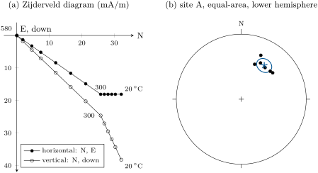
The directions of the specimens of a site scatter about a mean, and the statistics of that scatter are those of a distribution on the sphere.

Proposition 4.13 (Fisher distribution)

The Fisher distribution of precision parameter $\kappa > 0$ about a mean direction gives a unit vector the probability density, per unit solid angle,

$$f(\theta) = \frac{\kappa}{4\pi\sinh\kappa}\,e^{\kappa\cos\theta},$$

where $\theta$ is its angle from the mean. Given $N$ unit vectors $\mathbf u_i$ drawn from it, with resultant $\mathbf R = \sum\mathbf u_i$ of length $R$, the best estimate of the mean direction is that of $\mathbf R$; the precision is estimated by $k = (N - 1)/(N - R)$; and the true mean lies, with probability $1 - p$, within the angle $\alpha_{1-p}$ of the estimated mean, where

$$\cos\alpha_{1-p} = 1 - \frac{N - R}{R}\Bigl[\Bigl(\frac1p\Bigr)^{1/(N-1)} - 1\Bigr].$$

Definition 4.14 (Alpha-95)

The alpha-95 ($\alpha_{95}$) of a mean direction is the semi-angle of its cone of 95-per-cent confidence, the angle $\alpha_{1-p}$ of Proposition 4.13 for $p = 0.05$.

The density integrates to one: with $\mathrm d\Omega = 2\pi\sin\theta\,\mathrm d\theta$, $\int_0^\pi f\,2\pi\sin\theta\,\mathrm d\theta = \frac{\kappa}{2\sinh\kappa}\cdot\frac{e^\kappa - e^{-\kappa}}{\kappa} = 1$. Directions are averaged as unit vectors, never as angles: the mean of declinations $350{}^{\circ}$ and $10{}^{\circ}$ is north, not south. A large $k$ means a tight cluster, and $\alpha_{95}$ shrinks roughly as $1/\sqrt{kN}$.

Method 4.15 (Field tests of a palaeomagnetic direction)

A ChRM can be shown to predate an event by a test made in the field.

• Fold test. Sites on both limbs of a fold: if the directions cluster better after the beds are rotated back to horizontal than before, the magnetisation is older than the folding.
• Reversal test. If a formation holds both polarities, the mean of the reversed directions, inverted, should coincide with the mean of the normal ones within their confidence cones; a viscous overprint left unremoved would bias both in the same sense and break the antipodality.
• Baked-contact test. A dyke heats the host rock beside it, which acquires a new TRM: if the baked rock carries the dyke’s direction and the host rock further away a different one, the dyke’s magnetisation has not been reset since it cooled.

4.4 Poles and plates

If the field, averaged over a few thousand years to smooth out the secular variation, is a geocentric axial dipole, then the dipole formula turns a mean inclination into a latitude, and the mean declination points to the pole.

Definition 4.16 (Palaeolatitude; virtual geomagnetic pole)

The palaeolatitude of a site is the latitude $\lambda$ given by its mean inclination through the dipole formula, $\tan I = 2\tan\lambda$. The virtual geomagnetic pole (VGP) of a direction $(D, I)$ observed at a site is the north pole of the geocentric dipole that would produce that direction there.

Theorem 4.17 (The pole of a direction)

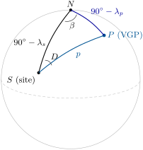
Let a site have latitude $\lambda_s$ and longitude $\varphi_s$ and a mean direction $(D, I)$. Let $p$ be the palaeocolatitude, $\cot p = \tfrac12\tan I$, with $0 \le p \le 180{}^{\circ}$. The virtual geomagnetic pole has latitude $\lambda_p$ and longitude $\varphi_p$ given by

$$\sin\lambda_p = \sin\lambda_s\cos p + \cos\lambda_s\sin p\cos D,\qquad \sin\beta = \frac{\sin p\sin D}{\cos\lambda_p},$$

with $\varphi_p = \varphi_s + \beta$ if $\cos p \ge \sin\lambda_s\sin\lambda_p$, and $\varphi_p = \varphi_s + 180{}^{\circ} - \beta$ otherwise.

The cone $\alpha_{95}$ about the mean direction becomes an oval about the pole, of semi-axes $\mathrm dp = \tfrac12\alpha_{95}(1 + 3\cos^2p)$ along the great circle from the site, and $\mathrm dm = \alpha_{95}\sin p/\cos I$ across it. A pole averaged over several sites of a formation, each a VGP, is a palaeomagnetic pole with its own cone, $A_{95}$. Rocks of the same age on one rigid plate give the same pole; rocks of different ages, different poles.

Definition 4.18 (Apparent polar wander; apparent polar wander path)

Apparent polar wander is the change, with the age of the rocks, of the palaeomagnetic pole of a plate seen from that plate, held fixed. An apparent polar wander path is the curve joining the palaeomagnetic poles of a plate in order of age.

The pole does not wander: the plate moves, and the path records that motion in reverse. Two plates that have moved apart have different paths for the time before their separation, and each path is rotated onto the other by the finite rotation that closes the ocean between them. A palaeomagnetic pole fixes the latitude of a block and its orientation, but not its longitude: a rotation of the block about the spin axis changes neither.

A displaced block, a terrane, is tested against the path of the stable plate it is now part of. From the reference pole of the right age one computes the expected direction $(D_x, I_x)$ at the site, by Theorem 4.17 read backwards. A clockwise rotation of the block about a vertical axis is measured by $R = D_o - D_x$, its poleward displacement by $P = \lambda_x - \lambda_o$, the difference between expected and observed palaeolatitudes; the error of a declination is about $\Delta D = \arcsin(\sin\alpha_{95}/\cos I)$, and errors combine as the root of the sum of their squares. The Hawaiian–Emperor chain was put to this test in the Year 1 volume, in its chapter on hotspots: the palaeolatitudes measured on the Emperor seamounts showed the hotspot itself moving south, by more than $40\,\mathrm{mm}/\mathrm{yr}$ from 81 to $47\,\mathrm{Ma}$.

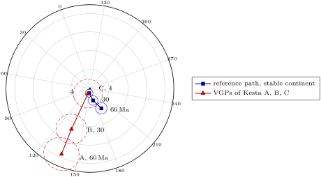
A pole that moves with respect to the spin axis can mean either that the plates moved or that the whole solid Earth turned beneath the spin axis.

Definition 4.19 (True polar wander)

True polar wander is the rotation of the whole solid Earth, mantle and crust together, with respect to its spin axis, driven by changes in the distribution of mass inside it. It moves all the palaeomagnetic poles of all the plates together, by the same rotation, whereas plate motion moves each plate’s poles differently.

It is detected only by comparing the paths of all the plates within a frame that is independent of the spin axis, such as that of the hotspots; how large it has been is still debated, and no rate is quoted here.

4.5 Magnetostratigraphy

Definition 4.20 (Magnetostratigraphy)

Magnetostratigraphy is the subdivision of a sequence of rocks into polarity zones, intervals of uniform normal or reversed polarity, and the dating of the sequence by matching its pattern of zones with that of the geomagnetic polarity timescale.

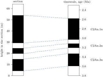
A reversal is recorded, within the resolution of the sampling, everywhere at the same time: a reversal boundary in a section is an isochronous surface. The pattern of zones, their number and their relative thicknesses, is what is matched; a single zone, alone, could be any chron of its polarity. One or two independent ages, from a volcanic ash or a fossil, anchor the match, and then every reversal boundary dates the section. In the figure below, a section of $64\,\mathrm{m}$ shows three normal zones; fitted to the normal subchrons of chron C2An, from 3.596 to $2.581\,\mathrm{Ma}$, its boundaries give an accumulation rate of about $40\,\mathrm{m}/\mathrm{Myr}$ below $20\,\mathrm{m}$ and $55\,\mathrm{m}/\mathrm{Myr}$ above.

In the lab — A shielded palaeomagnetic laboratory

The laboratory is a room inside a magnetic shield, layers of high-permeability metal that cut the Earth’s field to a small fraction of its value, so that the specimens acquire no new remanence while they are handled. A palaeomagnetist loads the specimens, small cylinders of rock each marked with an orientation arrow, onto a long tray that carries them, one after the other, into a cryogenic magnetometer, whose superconducting sensors, cooled by liquid helium, measure the three components of remanences far weaker than a compass could sense. Between measurements the specimens go into a shielded oven for the next heating step, or through the coils of an alternating-field demagnetiser attached to the same line, and the software plots each Zijderveld diagram as the steps accumulate.

4.6 Exercises

Exercise 4.1 ★

In a geocentric axial dipole field, compute the inclination at latitude $30{}^{\circ}$ N, and the latitude of a site where the inclination is $-20{}^{\circ}$.

Solution

Solution of Exercise 4.1.

$\tan I = 2\tan30{}^{\circ} = 1.1547$, so $I = 49.1{}^{\circ}$. Conversely, $\tan\lambda = \tfrac12\tan(-20{}^{\circ}) = -0.1820$, so $\lambda = -10.3{}^{\circ}$, that is $10.3{}^{\circ}$ S.

Exercise 4.2 ★

At a station, the field has components $X = 20\,000\,\mathrm{nT}$, $Y = -2000\,\mathrm{nT}$ and $Z = 40\,000\,\mathrm{nT}$. Compute $H$, $F$, the magnetic declination and the inclination.

Solution

Solution of Exercise 4.2.

$H = \sqrt{20000^2 + 2000^2} = 20\,100\,\mathrm{nT}$; $F = \sqrt{20000^2 + 2000^2 + 40000^2} = 44\,770\,\mathrm{nT}$. The magnetic declination is $\arctan(-2000/20000) = -5.7{}^{\circ}$, $5.7{}^{\circ}$ west of north; the inclination $\arctan(40000/20100) = 63.3{}^{\circ}$, downwards.

Exercise 4.3 ★

In 2025, $g_1^0 = -29\,350\,\mathrm{nT}$. Taking the field as an axial dipole, compute the field at the equator and at the poles, and the dipole moment ($a = 6371.2\,\mathrm{km}$, $\mu_0 = 4\pi\times10^{-7}\,\mathrm{H}\,\mathrm{m}^{-1}$).

Solution

Solution of Exercise 4.3.

$B_0 = -g_1^0 = 29\,350\,\mathrm{nT}$ at the equator, and $2B_0 = 58\,700\,\mathrm{nT}$ at the poles. $m = 4\pi a^3B_0/\mu_0 = a^3B_0/10^{-7} = 2.5862 \times 10^{20}\times 2.935 \times 10^{-5}/10^{-7} = 7.59 \times 10^{22}\,\mathrm{A}\,\mathrm{m}^{2}$, a little less than the $7.69 \times 10^{22}\,\mathrm{A}\,\mathrm{m}^{2}$ of the full dipole, which adds $g_1^1$ and $h_1^1$.

Exercise 4.4 ★

Name the kind of remanence acquired, and when it records the field, by: (a) a lava flow cooling; (b) silt settling in a quiet lake; (c) a sandstone whose iron oxide coatings turn to haematite during early burial; (d) a basalt sitting for a million years in the present field.

Solution

Solution of Exercise 4.4.

(a) A thermoremanent magnetisation, recording the field as the lava cooled through the blocking temperatures of its grains. (b) A detrital remanent magnetisation, recording the field within the time the silt took to settle and be locked by compaction. (c) A chemical remanent magnetisation, recording the field during the growth of the haematite, during early burial and so somewhat after deposition. (d) A viscous remanence along the present field, added to the original TRM by the grains of shortest relaxation time; it is removed by the first steps of demagnetisation.

Exercise 4.5 ★★

Four specimens of a site give the directions $(D, I)$: $(12{}^{\circ}, 48{}^{\circ})$, $(22{}^{\circ}, 44{}^{\circ})$, $(16{}^{\circ}, 57{}^{\circ})$ and $(6{}^{\circ}, 53{}^{\circ})$. Compute their unit vectors, the resultant length $R$, the mean direction, $k$ and $\alpha_{95}$.

Solution

Solution of Exercise 4.5.

The unit vectors $(\cos I\cos D,\ \cos I\sin D,\ \sin I)$ are

$$\begin{gather*} (0.6545, 0.1391, 0.7431),\quad (0.6670, 0.2695, 0.6947),\\ (0.5235, 0.1501, 0.8387),\quad (0.5985, 0.0629, 0.7986). \end{gather*}$$

The sum is $(2.4435, 0.6216, 3.0751)$, of length $R = 3.9766$. Mean: $D = \arctan(0.6216/2.4435) = 14.3{}^{\circ}$, $I = \arcsin(3.0751/3.9766) = 50.7{}^{\circ}$. $k = 3/(4 - 3.9766) = 128$. With $20^{1/3} - 1 = 1.7144$, $\cos\alpha_{95} = 1 - (0.0234/3.9766)\times1.7144 = 0.98991$, so $\alpha_{95} = 8.1{}^{\circ}$: with four specimens the cone stays wide, however tight the group.

Exercise 4.6 ★★

A site at $40.0{}^{\circ}$ N, $10.0{}^{\circ}$ E gives the mean direction $D = 20{}^{\circ}$, $I = 50{}^{\circ}$. Compute its palaeolatitude and its virtual geomagnetic pole.

Solution

Solution of Exercise 4.6.

$\lambda = \arctan(\tfrac12\tan50{}^{\circ}) = 30.79{}^{\circ}$, so $p = 59.21{}^{\circ}$. $\sin\lambda_p = \sin40{}^{\circ}\cos59.21{}^{\circ} + \cos40{}^{\circ}\sin59.21{}^{\circ} \cos20{}^{\circ} = 0.9474$, $\lambda_p = 71.34{}^{\circ}$ N. $\sin\beta = \sin59.21{}^{\circ}\sin20{}^{\circ}/\cos71.34{}^{\circ} = 0.9184$, $\beta = 66.66{}^{\circ}$. Since $\cos p = 0.5119 < \sin40{}^{\circ}\times0.9474 = 0.6090$, the second case applies: $\varphi_p = 10 + 180 - 66.66 = 123.34{}^{\circ}$ E. The pole is at $71.3{}^{\circ}$ N, $123.3{}^{\circ}$ E.

Exercise 4.7 ★★

The IGRF gives a dipole moment of $8.32 \times 10^{22}\,\mathrm{A}\,\mathrm{m}^{2}$ in 1900 and $7.69 \times 10^{22}\,\mathrm{A}\,\mathrm{m}^{2}$ in 2025, and a rate of change of $g_1^0$ of $+12.6\,\mathrm{nT}/\mathrm{yr}$ in 2025. (a) Compute the relative change of the moment per century. (b) If $g_1^0$ kept that rate, in how many years would it reach zero? Why is this not a forecast?

Solution

Solution of Exercise 4.7.

(a) $(7.69 - 8.32)/8.32 = -7.6\,\%$ in 125 years, or $-6.1\,\%$ per century. (b) $29350/12.6 = 2329$, about 2300 years. It is no forecast: the rate itself changes from one five-year model to the next, the moment has been both higher and lower in the past without reversing, and the field reverses at irregular intervals that no rate predicts.

Exercise 4.8 ★★

A specimen’s remaining remanence, in $\mathrm{mA}/\mathrm{m}$ (north, east, down), is $(32.2, 18.1, 38.2)$ after heating to $20\,{}^{\circ}\mathrm{C}$, $(25.8, 18.1, 24.6)$ after $300\,{}^{\circ}\mathrm{C}$, and $(0.0, 0.0, 0.0)$ after $580\,{}^{\circ}\mathrm{C}$; the Zijderveld diagram is straight between each pair. Compute the direction and intensity of the component removed between 20 and $300\,{}^{\circ}\mathrm{C}$ and of that removed above $300\,{}^{\circ}\mathrm{C}$. Which is the ChRM, and what is the other?

Solution

Solution of Exercise 4.8.

Between 20 and $300\,{}^{\circ}\mathrm{C}$ the vector lost $(6.4, 0.0, 13.6)$: a component of $15.0\,\mathrm{mA}/\mathrm{m}$, with $D = 0.0{}^{\circ}$ and $I = \arctan(13.6/6.4) = 64.8{}^{\circ}$. Above $300\,{}^{\circ}\mathrm{C}$ it lost $(25.8, 18.1, 24.6)$: $40.0\,\mathrm{mA}/\mathrm{m}$, $D = \arctan(18.1/25.8) = 35.1{}^{\circ}$, $I = \arctan(24.6/31.5) = 38.0{}^{\circ}$. The second, which goes to the origin, is the ChRM; the first, along a northward, steep direction, removed at low temperature, is a viscous overprint along the recent field.

Exercise 4.9 ★★

A formation gives $I = -35{}^{\circ}$ with $\alpha_{95} = 5{}^{\circ}$. Compute its palaeolatitude, the range of palaeolatitudes allowed by $I \pm \alpha_{95}$, and the semi-axes $\mathrm dp$ and $\mathrm dm$ of the confidence oval of its pole.

Solution

Solution of Exercise 4.9.

$\lambda = \arctan(\tfrac12\tan(-35{}^{\circ})) = -19.3{}^{\circ}$. For $I = -40{}^{\circ}$ and $-30{}^{\circ}$: $-22.8{}^{\circ}$ and $-16.1{}^{\circ}$, an interval of $6.7{}^{\circ}$. $p = 90{}^{\circ} - \lambda = 109.3{}^{\circ}$, $\cos^2p = 0.1096$: $\mathrm dp = 2.5\times(1 + 0.329) = 3.3{}^{\circ}$ and $\mathrm dm = 5\times\sin109.3{}^{\circ}/\cos35{}^{\circ} = 5.8{}^{\circ}$.

Exercise 4.10 ★★★

(a) From Theorem 4.3, find the latitude where the inclination is $45{}^{\circ}$, and the ratio of the field at the poles to that at the equator. (b) Show that $\mathrm dI/\mathrm d\lambda = 2/(1 + 3\sin^2\lambda)$, and deduce where an error of inclination gives the largest error of palaeolatitude. (c) Why are palaeolatitudes from low inclinations the most precise in degrees?

Solution

Solution of Exercise 4.10.

(a) $\tan\lambda = \tfrac12$, $\lambda = 26.6{}^{\circ}$. $F$ is $B_0$ at the equator and $2B_0$ at the poles: a ratio of 2. (b) $\tan I = 2\tan\lambda$ gives $(1 + \tan^2I)\,\mathrm dI = 2(1 + \tan^2\lambda)\,\mathrm d\lambda$, so

$$\frac{\mathrm dI}{\mathrm d\lambda} = \frac{2/\cos^2\lambda}{1 + 4\tan^2\lambda} = \frac{2}{\cos^2\lambda + 4\sin^2\lambda} = \frac{2}{1 + 3\sin^2\lambda}.$$

An error $\delta I$ gives $\delta\lambda = \tfrac12(1 + 3\sin^2\lambda)\,\delta I$, from $\tfrac12\delta I$ at the equator to $2\,\delta I$ at the poles: the largest error is near the poles. (c) Near the equator the inclination changes twice as fast as the latitude, so a given error of inclination costs half as much latitude; near the poles the inclination hardly changes with latitude.

Exercise 4.11 ★★★

A site lies at $35.0{}^{\circ}$ S, $150.0{}^{\circ}$ E on a stable plate whose reference pole, for the age of a formation sampled there, is at $70.0{}^{\circ}$ N, $300.0{}^{\circ}$ E. (a) Compute the angular distance $p$ from the site to the pole, the expected inclination and declination, and the expected palaeolatitude. (b) The formation gives $D_o = 30.0{}^{\circ}$, $I_o = -60.0{}^{\circ}$. Compute the rotation $R$ and the poleward displacement $P$, and say what they mean.

Solution

Solution of Exercise 4.11.

(a) $\cos p = \sin(-35{}^{\circ})\sin70{}^{\circ} + \cos35{}^{\circ}\cos70{}^{\circ}\cos150{}^{\circ} = -0.5390 - 0.2426 = -0.7816$, $p = 141.41{}^{\circ}$. Then $\tan I_x = 2\cot p = -2.506$, $I_x = -68.2{}^{\circ}$, and $\lambda_x = 90{}^{\circ} - p = -51.4{}^{\circ}$. $\cos D_x = (\sin70{}^{\circ} - \sin(-35{}^{\circ})\cos p)/(\cos35{}^{\circ}\sin p) = 0.9617$, and since the pole lies east of the site’s meridian ($\sin150{}^{\circ} > 0$), $D_x = 15.9{}^{\circ}$. (b) $\lambda_o = \arctan(\tfrac12\tan(-60{}^{\circ})) = -40.9{}^{\circ}$. $R = 30.0 - 15.9 = 14.1{}^{\circ}$: a clockwise rotation of the block about a vertical axis. $P = \lambda_x - \lambda_o = -51.4 + 40.9 = -10.5{}^{\circ}$: the formation lay $10.5{}^{\circ}$ further north than the stable plate says it should, so the block has since moved about $10.5{}^{\circ}$, some $1170\,\mathrm{km}$, southwards with respect to the plate.

Exercise 4.12 ★★★

(a) From Proposition 4.13, show that the probability that a direction lies within $\theta$ of the mean is $(e^\kappa - e^{\kappa\cos\theta})/(e^\kappa - e^{-\kappa})$. (b) For large $\kappa$ and small $\theta$, show that this is about $1 - e^{-\kappa\theta^2/2}$, and deduce that $63\,\%$ of the directions lie within $\theta_{63} \approx 81{}^{\circ}/\sqrt\kappa$. (c) Compute $\theta_{63}$ for $\kappa = 50$, and check the $63\,\%$ with the exact formula.

Solution

Solution of Exercise 4.12.

(a) With $\mathrm d\Omega = 2\pi\sin\theta'\,\mathrm d\theta'$,

$$\int_0^\theta\frac{\kappa e^{\kappa\cos\theta'}}{4\pi\sinh\kappa}\,2\pi\sin\theta'\, \mathrm d\theta' = \frac{e^\kappa - e^{\kappa\cos\theta}}{2\sinh\kappa} = \frac{e^\kappa - e^{\kappa\cos\theta}}{e^\kappa - e^{-\kappa}} .$$

(b) For large $\kappa$, $e^{-\kappa}$ is negligible; dividing by $e^\kappa$ leaves $1 - e^{-\kappa(1 - \cos\theta)} \approx 1 - e^{-\kappa\theta^2/2}$. It equals $1 - e^{-1} = 63\,\%$ when $\kappa\theta^2/2 = 1$, $\theta = \sqrt{2/\kappa}$ radians, or $81{}^{\circ}/\sqrt\kappa$. (c) $81/\sqrt{50} = 11.5{}^{\circ}$; the exact formula gives $63.1\,\%$.

4.7 Problem: The Red Beds of Kesta

Problem 4.1

Weekend problem — three formations of a displaced terrane, their directions, poles and rotations, and the age of the youngest

Kesta is an invented terrane, now at $47.0{}^{\circ}$ N, $15.0{}^{\circ}$ E, at the edge of an invented stable continent. It exposes three red-bed formations: A, $60\,\mathrm{Ma}$; B, $30\,\mathrm{Ma}$; C, from about 3.7 to $2.4\,\mathrm{Ma}$. Each was sampled at several sites, and every specimen was thermally demagnetised; the ChRM is carried by haematite, and the formations are horizontal.

Part I — Mean directions. The six sites of formation A give $(D, I)$: $(50{}^{\circ}, 37{}^{\circ})$, $(28{}^{\circ}, 37{}^{\circ})$, $(21{}^{\circ}, 42{}^{\circ})$, $(24{}^{\circ}, 27{}^{\circ})$, $(37{}^{\circ}, 39{}^{\circ})$, $(46{}^{\circ}, 38{}^{\circ})$.

1. Why may a ChRM carried by haematite in a red bed be younger than the bed? What would show that it is not much younger?
2. Compute the unit vector of the first direction.
3. The six unit vectors sum to $(3.8943, 2.6500, 3.5717)$. Compute $R$ and the mean direction of formation A.
4. Compute $k$ and $\alpha_{95}$ for formation A.
5. Formation B gives, from 7 sites, $D = 23.9{}^{\circ}$, $I = 51.5{}^{\circ}$ and $R = 6.8979$; formation C, from 8 sites, $D = 3.4{}^{\circ}$, $I = 63.7{}^{\circ}$ and $R = 7.8707$. Compute $k$ and $\alpha_{95}$ of each.
6. Which formation is the best grouped? Which mean is the best defined?

Part II — Palaeolatitudes and poles.

7. Compute the palaeolatitudes of A, B and C.
8. For formation A, compute the palaeocolatitude $p$ and the latitude of its virtual geomagnetic pole.
9. Compute the longitude of that pole, checking which case of Theorem 4.17 applies.
10. Compute $\mathrm dp$ and $\mathrm dm$ for the pole of A.
11. The poles of B and C are at $66.5{}^{\circ}$ N, $135.6{}^{\circ}$ E and $87.1{}^{\circ}$ N, $139.1{}^{\circ}$ E. Describe the path of the three poles with age.

Part III — The age of formation C. In formation C, from its base, the specimens are reversed up to $4.2\,\mathrm{m}$, normal to $14.8\,\mathrm{m}$, reversed to $19.7\,\mathrm{m}$, normal to $24.6\,\mathrm{m}$, reversed to $29.2\,\mathrm{m}$ and normal to $54.0\,\mathrm{m}$, then reversed to the top at $64.0\,\mathrm{m}$. An ash bed at $22\,\mathrm{m}$ is dated at about $3.2\,\mathrm{Ma}$. The normal subchrons of chron C2An span 3.596–3.330, 3.207–3.116 and 3.032–$2.581\,\mathrm{Ma}$.

12. Match the polarity zones with the timescale, using the ash bed.
13. Compute the accumulation rate between the first and the third reversal boundary, and between the fourth and the sixth.
14. Estimate the ages of the base and the top of the section.
15. Why is the rate a mean over hundreds of thousands of years, and what could make it change?

Part IV — Against the stable continent, and the drift. The reference poles of the stable continent are at $78.0{}^{\circ}$ N, $190.0{}^{\circ}$ E ($A_{95} = 3.0{}^{\circ}$) at $60\,\mathrm{Ma}$; $83.5{}^{\circ}$ N, $175.0{}^{\circ}$ E ($2.5{}^{\circ}$) at $30\,\mathrm{Ma}$; and $87.5{}^{\circ}$ N, $150.0{}^{\circ}$ E ($2.0{}^{\circ}$) at $4\,\mathrm{Ma}$.

16. Compute the angular distance from Kesta to the $60\,\mathrm{Ma}$ reference pole, and the expected inclination and palaeolatitude.
17. Compute the expected declination at $60\,\mathrm{Ma}$.
18. The expected directions at 30 and $4\,\mathrm{Ma}$ are $(2.9{}^{\circ}, 60.0{}^{\circ})$ and $(2.5{}^{\circ}, 63.6{}^{\circ})$. Compute the poleward displacement $P$ of A, B and C.
19. Compute the rotation $R$ of A, B and C.
20. Compute the errors $\Delta D_o$ and $\Delta D_x$ for A, and the error of its rotation.
21. The errors of $R$ for B and C are $13.8{}^{\circ}$ and $17.9{}^{\circ}$. Which rotations are significant at 95 per cent?
22. Tell the history of Kesta relative to the stable continent.
23. Compute Kesta’s northward drift since formation A, with respect to the spin axis, in degrees and in kilometres ($111.19\,\mathrm{km}$ per degree).
24. Compute the palaeolatitudes allowed by $I \pm \alpha_{95}$ for formation A, and take as one standard deviation half the width of that interval divided by 1.96. Give Kesta’s northward drift since formation A, in kilometres, with its standard deviation.

Solution

Solution of Problem 4.1.

1. Haematite in a red bed may grow from iron oxides and hydroxides long after the sediment was laid down, giving a chemical remanence of that later age. A positive fold test, if the beds were folded soon after deposition, or a positive reversal test across closely spaced beds of both polarities would show the remanence to be early.

2. $(\cos37{}^{\circ}\cos50{}^{\circ}, \cos37{}^{\circ}\sin50{}^{\circ}, \sin37{}^{\circ}) = (0.5134, 0.6118, 0.6018)$.

3. $R = \sqrt{3.8943^2 + 2.6500^2 + 3.5717^2} = 5.9114$. $D = \arctan(2.6500/3.8943) = 34.2{}^{\circ}$, $I = \arcsin(3.5717/5.9114) = 37.2{}^{\circ}$.

4. $k = 5/(6 - 5.9114) = 56.5$. With $20^{1/5} - 1 = 0.8206$, $\cos\alpha_{95} = 1 - (0.0886/5.9114)\times0.8206 = 0.98771$, $\alpha_{95} = 9.0{}^{\circ}$.

5. B: $k = 6/(7 - 6.8979) = 58.8$; $20^{1/6} - 1 = 0.6475$, $\cos\alpha_{95} = 1 - (0.1021/6.8979)\times0.6475 = 0.99042$, $\alpha_{95} = 7.9{}^{\circ}$. C: $k = 7/(8 - 7.8707) = 54.1$; $20^{1/7} - 1 = 0.5340$, $\cos\alpha_{95} = 1 - (0.1293/7.8707)\times0.5340 = 0.99123$, $\alpha_{95} = 7.6{}^{\circ}$.

6. B has the largest $k$, the tightest group; C has the smallest $\alpha_{95}$, the best-defined mean, because it has the most sites. The three are close: all three formations are well grouped.

7. $\lambda_A = \arctan(\tfrac12\tan37.17{}^{\circ}) = 20.76{}^{\circ}$ N, $\lambda_B = 32.15{}^{\circ}$ N, $\lambda_C = 45.33{}^{\circ}$ N.

8. $p = 90 - 20.76 = 69.24{}^{\circ}$. $\sin\lambda_p = \sin47{}^{\circ}\cos69.24{}^{\circ} + \cos47{}^{\circ}\sin69.24{}^{\circ}\cos34.23{}^{\circ} = 0.2593 + 0.5272 = 0.7865$: $\lambda_p = 51.86{}^{\circ}$ N.

9. $\sin\beta = \sin69.24{}^{\circ}\sin34.23{}^{\circ}/\cos51.86{}^{\circ} = 0.8516$, $\beta = 58.40{}^{\circ}$. Since $\cos p = 0.3545 < \sin47{}^{\circ}\times 0.7865 = 0.5752$, the second case applies, $\cos\beta < 0$: $\varphi_p = 15.00 + 180 - 58.40 = 136.60{}^{\circ}$ E.

10. $\cos^2p = 0.1257$: $\mathrm dp = 4.50\times1.377 = 6.2{}^{\circ}$; $\mathrm dm = 8.99\times\sin69.24{}^{\circ}/\cos37.17{}^{\circ} = 10.5{}^{\circ}$.

11. From $51.9{}^{\circ}$ N at $60\,\mathrm{Ma}$ to $66.5{}^{\circ}$ N at $30\,\mathrm{Ma}$ and $87.1{}^{\circ}$ N at $4\,\mathrm{Ma}$, on nearly the same meridian ($136{}^{\circ}$–$139{}^{\circ}$ E): a path towards the geographic pole, reached within its cone by the youngest formation.

12. The ash bed, at $22\,\mathrm{m}$, lies in the second normal zone, 19.7–$24.6\,\mathrm{m}$; with an age near $3.2\,\mathrm{Ma}$ that zone is C2An.2n (3.207–3.116). Then the zone 4.2–$14.8\,\mathrm{m}$ is C2An.3n, the zone 29.2–$54.0\,\mathrm{m}$ C2An.1n, the reversed base belongs to the chron below C2An, and the reversed top to the chron above it.

13. $(19.7 - 4.2)/(3.596 - 3.207) = 15.5/0.389 = 39.8\,\mathrm{m}/\mathrm{Myr}$; $(54.0 - 24.6)/(3.116 - 2.581) = 29.4/0.535 = 55.0\,\mathrm{m}/\mathrm{Myr}$.

14. Base: $3.596 + 4.2/39.8 = 3.70\,\mathrm{Ma}$. Top: $2.581 - 10.0/55.0 = 2.40\,\mathrm{Ma}$.

15. Only reversal boundaries are dated, a few hundred thousand years apart; between them the rate is assumed constant. A change of subsidence, of sediment supply or of climate, or a gap in deposition, would change it, and a hiatus could even remove a short zone and mislead the match.

16. $\cos p = \sin47{}^{\circ}\sin78{}^{\circ} + \cos47{}^{\circ}\cos78{}^{\circ} \cos175{}^{\circ} = 0.7154 - 0.1413 = 0.5741$, $p = 54.96{}^{\circ}$. $\tan I_x = 2\cot p = 1.4023$, $I_x = 54.5{}^{\circ}$; $\lambda_x = 35.04{}^{\circ}$ N.

17. $\cos D_x = (\sin78{}^{\circ} - \sin47{}^{\circ}\times0.5741)/ (\cos47{}^{\circ}\sin54.96{}^{\circ}) = 0.99976$; the pole lies east of the site’s meridian ($\sin175{}^{\circ} > 0$), so $D_x = 1.3{}^{\circ}$.

18. Expected palaeolatitudes from $I_x$ = $54.5{}^{\circ}$, $60.0{}^{\circ}$ and $63.6{}^{\circ}$: $35.03{}^{\circ}$, $40.89{}^{\circ}$ and $45.21{}^{\circ}$. $P_A = 35.03 - 20.76 = 14.3{}^{\circ}$, $P_B = 40.89 - 32.15 = 8.7{}^{\circ}$, $P_C = 45.21 - 45.33 = -0.1{}^{\circ}$.

19. $R_A = 34.2 - 1.3 = 32.9{}^{\circ}$, $R_B = 23.9 - 2.9 = 21.0{}^{\circ}$, $R_C = 3.4 - 2.5 = 0.9{}^{\circ}$, all clockwise.

20. $\Delta D_o = \arcsin(\sin8.99{}^{\circ}/\cos37.17{}^{\circ}) = 11.3{}^{\circ}$; $\Delta D_x = \arcsin(\sin3.0{}^{\circ}/\cos54.5{}^{\circ}) = 5.2{}^{\circ}$; $\Delta R_A = \sqrt{11.3^2 + 5.2^2} = 12.4{}^{\circ}$.

21. $R_A = 32.9{}^{\circ} \pm 12.4{}^{\circ}$ and $R_B = 21.0{}^{\circ} \pm 13.8{}^{\circ}$ are significant; $R_C = 0.9{}^{\circ} \pm 17.9{}^{\circ}$ is not.

22. Sixty million years ago Kesta lay about $14{}^{\circ}$ of latitude south of where the stable continent puts it, and was turned about $33{}^{\circ}$ anticlockwise from its present orientation. By $30\,\mathrm{Ma}$ it had come about $6{}^{\circ}$ of those $14{}^{\circ}$ north and turned $12{}^{\circ}$ of those $33{}^{\circ}$ clockwise; by $4\,\mathrm{Ma}$ it had reached its present place on the continent, with no rotation left. It drifted north along the continent’s margin, turning clockwise as it went, and was in place by $4\,\mathrm{Ma}$.

23. $47.00 - 20.76 = 26.24{}^{\circ}$, or $26.24\times111.19 = 2918\,\mathrm{km}$. This includes the motion of the stable continent itself; relative to it, Kesta moved $P_A = 14.3{}^{\circ}$.

24. $I = 28.18{}^{\circ}$ and $46.16{}^{\circ}$ give $\lambda = 15.00{}^{\circ}$ and $27.50{}^{\circ}$: a half-width of $6.25{}^{\circ}$, and one standard deviation of $6.25/1.96 = 3.19{}^{\circ}$, or $355\,\mathrm{km}$. Since formation A, Kesta has drifted northwards by $(2918 \pm 355)\,\mathrm{km}$.