University Earth and Space Sciences — Year 3 · 本科三年级
6Mantle Convection and Plate Driving Forces
The coast of northern Sweden rises out of the sea by about a centimetre a year, ten thousand years after the ice sheet that covered it melted away; the shores of Hudson Bay rise as fast. Nothing pushes them up but the mantle, slowly flowing back beneath the place the ice had pressed down. The rate at which the ground springs back weighs the viscosity of the mantle, and the same viscosity sets how fast the mantle convects and the plates move. This chapter asks why the solid mantle convects at all, how fast it must flow to carry the Earth’s heat, what forces move the plates, and what the rebound of the ground says about the mantle’s viscosity.
You already know
Viscosity, the creeping flow of a viscous fluid (the Stokes equations ∇p=η∇2u, ∇⋅u=0), Stokes’ law for a sphere, the Reynolds number and buoyancy are in the physics books’ university volumes. Mantle convection and isostatic rebound were met in the high-school volume (Grade 12), ridge push and slab pull in its Grade 11 part. The thermal boundary layer, the thermal lithosphere and the mantle adiabat are in the Year 1 volume, in its chapter on the Earth’s heat budget; hotspots, mantle plumes and large igneous provinces in its chapter on hotspots. The half-space cooling model is in Chapter 5, flexure of the lithosphere in Chapter 3, seismic tomography in Chapter 1.
6.1 Why the mantle convects
The mantle is solid: it carries S waves. Over millions of years, however, it creeps like a fluid of enormous viscosity, and a layer of fluid heated from below and cooled from above may stay at rest, the heat crossing it by conduction, or overturn. A blob of hot fluid of size d, lighter than its surroundings by ραΔT, rises at a speed of order ρgαΔTd2/η; it loses its heat by diffusion in a time of order d2/κ. If it can rise across the layer before it has cooled, the layer overturns.
Definition 6.1(Rayleigh number)
For a fluid layer of thickness d, density ρ, thermal expansion coefficient α, thermal diffusivity κ and viscosity η, under gravity g, with a temperature difference ΔT between its base and its top, the Rayleigh number is
Ra=κηρgαΔTd3,
the ratio of the diffusion time d2/κ to the buoyant rise time η/(ρgαΔTd).
Definition 6.2(Critical Rayleigh number)
The critical Rayleigh numberRac of a layer is the value of the Rayleigh number above which a small disturbance of the state of rest grows into convection, and below which it dies away.
Proposition 6.3(Onset of convection)
For a layer whose top and bottom are free of shear stress and held at fixed temperatures, a disturbance of horizontal wavenumber k (in units of 1/d) grows when Ra>(π2+k2)3/k2. The minimum of the right-hand side, at k=π/2, gives
Rac=427π4≈657.5,
and the first cells to appear are 22d wide. Between rigid boundaries, Rac≈1708.
Proof.Admitted at this level.∎
The linear stability analysis behind it, a perturbation of the heat and Stokes equations about the conductive state, is in the physics books’ treatment of convection; exercise 11 checks the minimum.
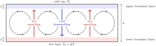
The figure below shows the convecting layer. The mantle’s values, with the depth of the core–mantle boundary, d=2891km, the mean density of the mantle, 4476kgm−3, and g between 9.8 and 10.7ms−2, all from the seismic Earth model PREM; α=3.1×10⁻⁵K−1 and ΔT=1450K from the plate model of Chapter 5; κ=10−6m2s−1; and η between 1021 and 1022Pas (Section 6.5), give Ra between 4.9×10⁶ and 4.9×10⁷, some seven thousand to seventy thousand times critical. The mantle cannot help convecting.
Convection in a layer heated from below and cooled from above. Heat crosses the thin boundary layers, of thickness δ, by conduction; in between, the well-mixed interior carries it by flow. Cold sheets detach from the upper layer and sink; hot ones rise from the lower.
The mantle is also heated from within, by the decay of radioactive elements, and from below, by the core. A layer heated only from within has no hot boundary layer at its base: its flow is driven by cold sheets sinking from the top, the rising flow being a broad, passive return. Slabs are such sheets, and plumes need the heat from the core.
6.2 Boundary layers and the strength of convection
Definition 6.4(Nusselt number)
The Nusselt number of a convecting layer is the heat flow through it divided by the heat flow that conduction alone would carry across the same layer, Nu=qd/(kΔT).
Theorem 6.5(Boundary-layer scaling of convection)
In a layer convecting at Ra≫Rac, if each thermal boundary layer grows until its own Rayleigh number, built on its thickness δ and the temperature drop ΔT/2 across it, reaches Rac, then
where u is the velocity scale of the flow, defined by requiring that the layer grows to δ while the fluid crosses the cell. This is the boundary-layer scaling of convection.
Proof. The interior is well mixed, at the mean temperature, so each boundary layer carries half of ΔT. Its Rayleigh number is ρgα(ΔT/2)δ3/(κη)=Ra(δ/d)3/2; setting it equal to Rac gives δ. The heat flow is conducted across the layer, q=k(ΔT/2)/δ, so Nu=qd/(kΔT)=d/(2δ). A boundary layer grows by diffusion to the thickness δ in a time δ2/κ; the fluid at the top crosses the cell, of width of order d, in a time d/u. Equating the two times, u=κd/δ2=(κ/d)(d/δ)2. ∎
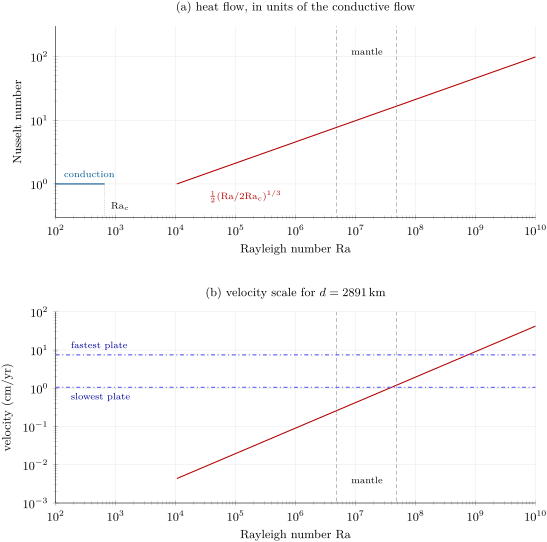
The heat flow grows only as the cube root of Ra: a hundred times lower viscosity, less than five times more heat. With the mantle’s Ra=4.9×10⁷, the scaling gives δ≈87km, Nu≈17, a heat flow of NukΔT/d≈26mWm−2 with k=3.1Wm−1K−1, and u≈1.2cm/yr (figure below). The boundary layer is as thick as the oceanic plate of Chapter 5, 95km; the root-mean-square speeds of today’s plates range from 1.1cm/yr (South America) to 7.5cm/yr (Cocos), 4.4cm/yr for the whole lithosphere. The Earth’s mean heat flow, 92mWm−2, is three to four times the scaling’s: the heat produced within the mantle, which a layer heated from below leaves out, and the constants of order one that the scaling ignores both weigh in. For a law with a single input, the orders of magnitude are right: plates are the upper boundary layer of a mantle with Ra∼107.
Convection scaling. (a) Below Rac the layer conducts (Nu=1); far above it, the boundary-layer law, drawn from Ra=16Rac≈1.1×10⁴, where it gives Nu=1 (in between, convection sets in gradually). (b) The velocity scale for the depth of the mantle and κ=10−6m2s−1, with the range of today’s plate speeds (dash-dotted). The dashed lines bound the mantle’s Rayleigh number for viscosities of 1022 and 1021Pas.
6.3 The forces on a plate
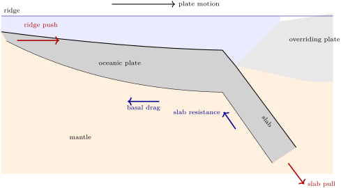
A plate moves at a steady speed: the forces on it balance. Three drive it or resist it from its edges and its base (figure below). The force that the sinking slab exerts on its plate, slab pull, comes from the excess density of a cold slab in the warmer mantle. Ridge push, the push of the high, hot ridge on the cooler plate beside it, follows from the half-space model of Chapter 5.
The forces on an oceanic plate: ridge push and slab pull drive it (red); drag at its base, where the plate moves faster than the mantle beneath, and the viscous resistance of the mantle to the sinking slab resist it (blue).
Proposition 6.6(Ridge-push force)
In the half-space cooling model, with mantle temperature Tm, surface temperature T0 and isostatic compensation, the horizontal force per unit length of ridge that the column at the ridge exerts on the plate of age t, the ridge-push force, is
Proof. Let y be the depth below the sea floor at the ridge, w the subsidence of the floor of age t, θ(z)=Tm−T(z) the temperature deficit at the depth z=y−w in its plate, and Θ(z)=∫0zθ. The ridge column holds mantle of density ρm from y=0; the old column holds water down to w, then plate of density ρm(1+αθ). The lithostatic pressures differ by Pr−Pt=(ρm−ρw)gy for y<w, and below,
Pr−Pt=(ρm−ρw)gw−ρmgαΘ(z)=ρmgα(Θ(∞)−Θ(z)),
by isostasy, (ρm−ρw)w=ρmαΘ(∞). The force is the integral of the pressure difference over depth; integrating the second part by parts,
Frp=21(ρm−ρw)gw2+ρmgα∫0∞zθ(z)dz.
For the half-space, θ=(Tm−T0)erfc(z/2κt) and ∫0∞xerfcxdx=1/4, so the integral is (Tm−T0)κt; and w=2ρmα(Tm−T0)κt/π/(ρm−ρw). Adding the two terms gives the formula. ∎
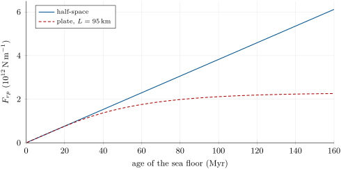
Ridge push grows linearly with age: it is not a push at the axis but a pressure gradient spread over the whole cooling plate. With the values of Chapter 5, the bracket is 1.04 and Frp=3.8×10¹²Nm−1 at 100Myr. In the plate model it stops growing with the depth, at about 2.3×10¹²Nm−1 (figure below). Slab pull is larger: a slab 95km thick, on average (Tm−T0)/2 colder than the mantle, hence denser by ρmα(Tm−T0)/2≈74kgm−3, hanging down to 670km, weighs 4.6×10¹³Nm−1 more than the mantle it displaces, twelve times the ridge push. Much of that weight is spent on the viscous mantle that resists the slab’s sinking, and only a part reaches the plate.
Ridge-push force against the age of the plate, from the two cooling models of Chapter 5, by numerical integration of the pressure difference (the half-space curve is the closed form of the proposition).
Definition 6.7(Basal drag)
Basal drag is the shear force per unit area that the mantle beneath a plate exerts on the plate’s base. For a plate moving at u over a layer of thickness h and viscosity η whose base is at rest, it is ηu/h, opposed to the motion; it drives the plate where the mantle beneath moves faster than the plate.
Which forces matter can be read from the plates themselves. The torque balance on each plate, fitted to plate motions, says that the forces acting on the sinking slab control the speed of oceanic plates and are about ten times stronger than any other, and that the resistance at the base is larger beneath continents than beneath oceans. The speeds agree: the fastest plates, Cocos at 75mm/yr, Nazca at 70 and the Pacific at 66mm/yr, are oceanic plates whose edges sink in long trenches; the slowest carry large continents, Eurasia at 23, North America at 20, South America at 11mm/yr.
6.4 Plumes
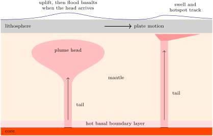
Hot sheets rising from the base of the mantle collect into columns: the mantle plumes of the Year 1 volume, with a large head and a thin tail (figure below). The swell of a hotspot, a broad rise of the sea floor around and downstream of the volcanoes, measures how much buoyancy its plume brings.
Definition 6.8(Plume buoyancy flux)
The plume buoyancy fluxB is the mass deficit, relative to the surrounding mantle, that a plume carries up per unit time; for a plume of volume flux Qv and temperature excess ΔT, B=ραΔTQv.
Proposition 6.9(Buoyancy flux from a swell)
If a plate moving at the speed u over a plume carries a swell of cross-sectional area A across the track, held up isostatically by the plume material beneath it, the plume’s buoyancy flux is
B=(ρm−ρw)Au.
Proof. By isostasy, a slice of swell of unit length along the track, which raises the sea floor over the area A of the cross-section and replaces water by rock, is held up by a mass deficit (ρm−ρw)A in the column beneath. The plate carries the slice away at the speed u, so in steady state the plume must supply the deficit for a length u of new swell per unit time. ∎
From the cross-sections of swells, the buoyancy fluxes of hotspots range over a factor of twenty: Hawaii, the largest, 8.7Mg/s; Iceland 1.4Mg/s; 37 hotspots together, about 50Mg/s. Each kilogram of buoyancy is cp/α joules of excess heat, so the heat flux is cpB/α; with cp=k/(ρmκ)=1170Jkg−1K−1 and α=3.1×10⁻⁵K−1, the 37 hotspots carry about 1.9TW, or 3.7mWm−2 over the Earth’s 5.1×10¹⁴m2, close to the 4mWm−2 published with the fluxes: a few per cent of the 47TW the Earth loses. Plumes are the minor partner of the heat budget; the plates carry the rest.
A young plume (left) rises as a large head fed by a thin tail; when the head spreads beneath the lithosphere, the surface rises and flood basalts may erupt. An older plume (right) is a tail beneath a moving plate, feeding a swell and a hotspot track. Not to scale.
A plume head is a sphere of buoyant mantle rising through the viscous mantle: physics’ Stokes law, v=2Δρga2/(9η), gives its speed in order of magnitude, a fraction of a metre a year for a head a few hundred kilometres across (exercise 8), so that it crosses the mantle in millions of years.
6.5 Glacial isostatic adjustment and the viscosity of the mantle
Glacial isostatic adjustment (GIA) is the slow deformation of the solid Earth, and the change of its gravity field and of sea level, as it returns towards isostatic equilibrium after an ice sheet grows or melts. The mantle viscosity is the effective viscosity η that relates the slow, steady creep of the mantle to the stresses that drive it, over times of thousands of years and more.
When an ice sheet melts, the depression it leaves is out of isostatic equilibrium: beneath it, the mantle’s pressure is lower than around it, and mantle flows in to lift the floor back. Today the coast of the Gulf of Bothnia rises at up to 10.3mm/yr, near Umeå; Hudson Bay at about 10mm/yr, where the ice was thickest, while the land south of the Great Lakes sinks by 1 to 2mm/yr, as the bulge that the ice had pushed up around it subsides. On the coasts, old shorelines now stand above the sea, the raised beaches of the field box below.
Theorem 6.11(Relaxation of a viscous half-space)
A depression w(x,t)=wm(t)cos(2πx/λ) of the surface of a half-space of uniform viscosity η and density ρ, left without load, decays as wm(t)=wm(0)e−t/τ with
τ=ρgλ4πη.
Proof. Take z downwards, k=2π/λ, and look for a Stokes flow that decays with depth, with vertical velocity (downwards) v=(C+Dkz)e−kzcoskx. Incompressibility gives the horizontal velocity u=−(D−C−Dkz)e−kzsinkx. These functions satisfy ∇4=0, as every Stokes flow in two dimensions does. The free surface carries no shear stress: ∂u/∂z+∂v/∂x=2k(D−C)sinkx=0 at z=0, so D=C, and
the pressure following from ∂p/∂x=η∇2u=−2ηCk2e−kzsinkx (and ∂p/∂z=η∇2v checks). At the surface ∂v/∂z=0, so the normal stress there is −p. Beneath a depression w, the weight of the missing rock lowers the pressure by ρgw: p(0)=−ρgw, so 2ηCk=−ρgwm. The surface moves with the fluid: dwm/dt=v(0)=C=−ρgwm/(2ηk), whose solution decays with τ=2ηk/(ρg)=4πη/(ρgλ). ∎
Definition 6.12(Isostatic relaxation time)
The isostatic relaxation timeτ of a load of horizontal scale λ is the time in which its departure from isostatic equilibrium decays by the factor e.
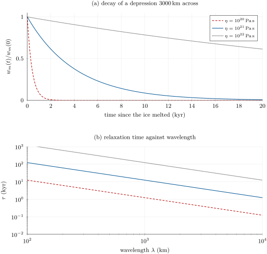
A uniform half-space relaxes broad depressions faster than narrow ones, and the flow beneath a load of wavelength λ decays with depth as e−kz, over a depth λ/2π: a large ice sheet stirs the mantle deeply, a small lake only its top. For a depression 3000km across and η=1021Pas, with ρ=3300kgm−3, τ=4.1kyr (figure below): after ten thousand years, e−2.4=9% of the depression remains, and since w˙=−w/τ, an uplift of 10mm/yr means that some 40m of rise are still to come.
Relaxation of a uniform viscous half-space (ρ=3300kgm−3, g=9.8ms−2) for three viscosities. (a) The fraction of the depression left with time. (b) The relaxation time 4πη/(ρgλ), longer for narrow loads.
The real mantle is not uniform, and its rebound is read with models that layer it and add an elastic lithosphere, which holds up narrow loads by flexure. The first estimate, from the rebound of Fennoscandia, gave 1021Pas, and the decay of uplift at the Angerman River in Sweden and at Richmond Gulf on Hudson Bay gives an average of 0.65 to 1.1×10²¹Pas from the base of the lithosphere down to about 1400km, with the upper mantle about ten times less viscous than the lower. Inversions of the GNSS uplift rates of Fennoscandia give upper-mantle viscosities of 5×10²⁰ to 1021Pas in one study and 3.4×10²⁰ to 5.0×10²⁰Pas in another, lower-mantle viscosities of 5×10²¹ to 5×10²²Pas, and a lithosphere 93 to 110km thick. The estimates differ by factors of two or three, but they agree on the order of magnitude and on the increase with depth.
Definition 6.13(Maxwell time)
The Maxwell time of a material of viscosity η and shear modulus μ is τM=η/μ: loads applied for much less than τM meet an elastic solid, loads applied for much longer a viscous fluid.
With μ=ρvS2=7.7×10¹⁰Pa at 300km in PREM and η=1021Pas, τM=1.3×10¹⁰s, about four hundred years. A seismic wave, which lasts seconds, crosses an elastic mantle; an ice age, and convection, deform a fluid one. The same rock is both, depending on how long it is pushed.
In the field— Raised beaches
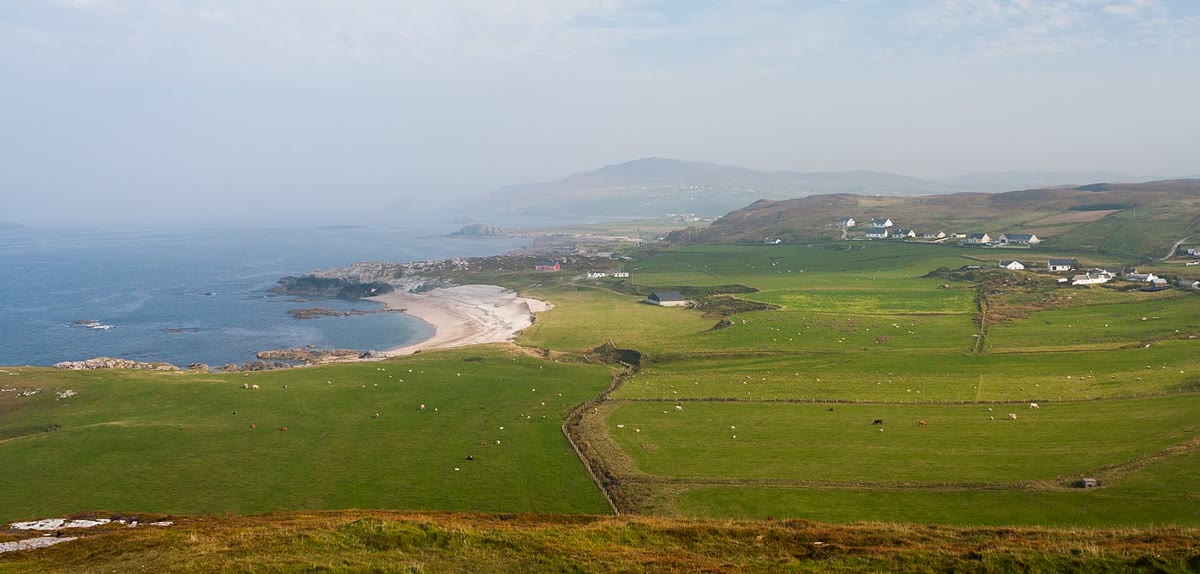
The raised beaches of Ballyhillin, Malin Head, in the north of Ireland: shingle ridges of old shorelines lifted above the sea as the land rose after its ice sheet melted. Photo A. F. Borchert, CC BY-SA 4.0.
On the coasts of formerly glaciated lands, a geomorphologist finds the sea’s old work stranded inland: ridges of rounded shingle, notches and flat platforms cut by waves, now standing above the reach of today’s highest tides, sometimes in a staircase of several levels. Each level was a shoreline when the sea stood there; the land has risen since. Shells and driftwood in the old beaches are dated by radiocarbon, and the heights of the dated levels, levelled to a benchmark, give the uplift against time. Traced along a coast, an old shoreline is found to slope, highest where the ice was thickest: the tilt maps the shape of the rebound.
6.6 Whole-mantle convection and its deep structure
Does the mantle convect as one layer, or as two, above and below the 670km discontinuity? Tomography (Chapter 1) answers in part: some slabs flatten above the discontinuity, others plunge through it into the lower mantle, so mass crosses it and the two layers are not sealed from each other. The increase of viscosity with depth makes the lower mantle flow more sluggishly, and slabs slow and thicken as they enter it.
At the base of the mantle, tomography shows two broad regions of low S-wave speed, beneath Africa and beneath the Pacific, the large low-shear-velocity provinces (LLSVPs). They are probably chemically distinct from the mantle above them and denser, piles rather than hot plumes. The large igneous provinces and kimberlites of the last few hundred million years erupted mostly above their margins, as if plumes rose from the edges of the piles, where the hot boundary layer at the base of the mantle is swept against them.
6.7 Exercises
Exercise 6.1★
Compute the Rayleigh number of an upper-mantle layer 670km thick with ρ=3500kgm−3, g=9.9ms−2, α=3×10⁻⁵K−1, ΔT=1000K, κ=10−6m2s−1 and η=5×10²⁰Pas. How many times critical is it, for free-slip boundaries?
Solution
Solution of Exercise 6.1.
Ra=3500×9.9×3×10−5×1000×(6.7×105)3/(10−6×5×1020)=6.25×105, about 950 times the critical 657.5: the layer convects vigorously.
Exercise 6.2★
Compute the Maxwell time of a mantle of viscosity 1021Pas and shear modulus 7.7×10¹⁰Pa, in years. Does the mantle respond elastically or viscously to the twice-daily Earth tide, to the melting of an ice sheet, and to the sinking of a slab?
Solution
Solution of Exercise 6.2.
τM=1021/7.7×1010=1.30×1010s, about 412yr. The tide, which lasts hours, meets an elastic mantle; the melting of an ice sheet, over thousands of years, and the sinking of a slab, over millions, meet a viscous one.
Exercise 6.3★
With η=1021Pas, ρ=3300kgm−3 and g=9.8ms−2, compute the relaxation time of a uniform half-space for loads of wavelength 1000 and 3000km. Which recovers faster?
Solution
Solution of Exercise 6.3.
τ=4π×1021/(3300×9.8λ): 3.89×10¹¹s = 12.3kyr for 1000km, and 4.1kyr for 3000km. The broader load recovers faster.
Exercise 6.4★
With g=9.8ms−2, ρm=3300kgm−3, ρw=1030kgm−3, α=3.1×10⁻⁵K−1, Tm−T0=1450K, κ=0.8×10⁻⁶m2s−1 and 1Myr=3.156×10¹³s, compute the ridge-push force at 50Myr. How many times smaller is it than a slab pull of 4.6×10¹³Nm−1?
Solution
Solution of Exercise 6.4.
gρmα(Tm−T0)κt=9.8×3300×3.1×10−5×1450×0.8×10−6×50×3.156×1013=1.835×10¹²Nm−1; the bracket is 1+2×3300×3.1×10−5×1450/(π×2270)=1.0416, so Frp=1.91×10¹²Nm−1, 24 times smaller than the slab pull.
Exercise 6.5★★
A blob of mantle 10km across, 300K hotter than its surroundings, rises at the speed ρgαΔTd2/η (take ρ=3300kgm−3, g=9.8ms−2, α=3×10⁻⁵K−1, η=1021Pas, κ=10−6m2s−1). (a) Compute its rise time across its own size and its diffusion time d2/κ, and show that their ratio is its Rayleigh number. (b) Does it rise or cool first? (c) How large must it be for its Rayleigh number to reach 657.5?
Solution
Solution of Exercise 6.5.
(a) v=3300×9.8×3×10−5×300×(104)2/1021=2.91×10−11ms−1; the rise time across 10km is d/v=3.44×1014s, 10.9Myr, the diffusion time d2/κ=1014s, 3.2Myr. Their ratio is (d2/κ)/(d/v)=vd/κ=ρgαΔTd3/(κη)=Ra=0.29. (b) It cools first: small blobs do not convect. (c) Ra∝d3, so d=10×(657.5/0.291)1/3=131km.
Exercise 6.6★★
For a layer 2891km deep at Ra=107, with κ=10−6m2s−1, k=3.1Wm−1K−1, ΔT=1450K and Rac=657.5, compute the boundary-layer thickness, the Nusselt number, the velocity scale in cm/yr and the heat flow.
Solution
Solution of Exercise 6.6.
2Rac=1315 and Ra/2Rac=7604, whose cube root is 19.66. δ=2891/19.66=147km, Nu=19.66/2=9.8, u=(10−6/2.891×106)×19.662=1.34×10−10ms−1=0.42cm/yr, and q=9.8×3.1×1450/2.891×106=15mWm−2.
Exercise 6.7★★
An invented hotspot swell has a cross-sectional area of 8×10⁸m2 across the track, and the plate above moves at 9cm/yr. With ρm−ρw=2270kgm−3, compute its buoyancy flux, and its heat flux with cp=1170Jkg−1K−1 and α=3.1×10⁻⁵K−1. What fraction of the Earth’s 46.7TW is it?
Solution
Solution of Exercise 6.7.
u=0.09/3.156×107=2.85×10−9ms−1 and B=2270×8×108×2.85×10−9=5.18×10³kgs−1=5.2Mg/s, about three-fifths of Hawaii’s. The heat flux is 1170×5178/3.1×10−5=1.95×1011W, 0.2TW, or 0.42% of the Earth’s heat loss.
Exercise 6.8★★
A plume head of radius 400km, lighter than the mantle by 30kgm−3, rises through a mantle of viscosity 1021Pas. With Stokes’ law, compute its speed in m/yr and the time it takes to rise 2000km.
Solution
Solution of Exercise 6.8.
v=2×30×9.8×(4×105)2/(9×1021)=1.05×10−8ms−1=0.33m/yr; 2000km take 2×10⁶/1.05×10−8=1.9×1014s, about 6Myr.
Exercise 6.9★★
A region was depressed by 300m when its ice melted, 10kyr ago, and relaxes with τ=4.4kyr. Compute the depression left today and the present uplift rate. Compare with the 10.3mm/yr measured near Umeå.
Solution
Solution of Exercise 6.9.
w=300e−10/4.4=30.9m and w˙=w/τ=30.9/4400=7.0mm/yr, two-thirds of the rate measured near Umeå: a uniform half-space with this τ is in the right range, but the real rebound is faster or its depression deeper.
Exercise 6.10★★★
(a) From the expression of Frp in the proof of Proposition 6.6, show that the first term, 21(ρm−ρw)gw2, is the second term of the bracket. (b) Show that ∫0∞xerfcxdx=1/4, by integrating by parts. (c) With the values of exercise 4, compute the two terms at 100Myr.
(b) By parts, ∫0∞xerfcxdx=[2x2erfcx]0∞+∫0∞2x2π2e−x2dx=0+π1⋅4π=41. (c) At 100Myr, ρmgα∫zθ=3.67×10¹²Nm−1 and, with w=3705m, 21(ρm−ρw)gw2=1.53×10¹¹Nm−1: the water term is only 4% of the force.
Exercise 6.11★★★
Show that f(k)=(π2+k2)3/k2 is smallest at k=π/2, where it equals 27π4/4. Deduce the width of a pair of convection cells at onset, in units of d, and the width of one cell.
Solution
Solution of Exercise 6.11.
lnf=3ln(π2+k2)−2lnk, whose derivative 6k/(π2+k2)−2/k vanishes when 3k2=π2+k2, k2=π2/2. There f=(3π2/2)3/(π2/2)=27π4/4. The wavelength 2π/k=22d=2.83d holds a pair of counter-rotating cells, each 2d=1.41d wide.
Exercise 6.12★★★
A plate 6000km long moves at 6cm/yr over a mantle layer 150km thick, of viscosity 1020Pas, whose base is at rest. (a) Compute the basal drag in MPa and the drag force per unit length of plate. (b) Compare with a ridge push of 3.8×10¹²Nm−1 and a slab pull of 4.6×10¹³Nm−1. (c) If one tenth of the slab pull reaches the plate, at what speed does the drag balance the driving forces?
Solution
Solution of Exercise 6.12.
(a) u=1.90×10⁻⁹ms−1, ηu/h=1020×1.90×10−9/1.5×105=1.27MPa, and over 6000km, 7.6×10¹²Nm−1. (b) Twice the ridge push and a sixth of the slab pull: the drag can resist the ridge push alone, but not the slab. (c) ηuL/h=3.8×1012+4.6×1012 gives u=8.4×1012×1.5×105/(6×106×1020)=2.1×10−9ms−1=6.6cm/yr, the speed of the fast oceanic plates.
6.8 Problem: Rebound of Lake Ardo
Problem 6.1
Weekend problem — the rebound of an invented lake basin, the viscosity of the mantle beneath it, and the convection that viscosity allows
Lake Ardo, an invented lake, filled a basin 250km across, dammed by an ice sheet, and stood 300m deep for about fifty thousand years. Fourteen thousand years ago the ice dam failed and the lake drained in a few weeks. Its highest shoreline, level when it formed, is now tilted; dated shorelines of the small lakes left in the basin give the uplift of the centre since the drainage, relative to the rim, which barely moved:
time since the drainage (kyr)
1
2
4
6
9
14
uplift of the centre (m)
11.5
21.6
38.0
50.5
64.0
77.2
Take ρw=1000kgm−3, ρm=3300kgm−3, g=9.8ms−2, 1yr=3.156×10⁷s, and treat the mantle as a uniform viscous half-space.
Part I — The load.
Compute the pressure of the lake on its floor.
Compute the depression of the floor at isostatic equilibrium, and say why the density of the mantle, not of the crust, appears in it.
Treating the lake as a disc, compute the mass of its water.
Explain why the highest shoreline is now tilted, and compute its mean slope from the rim to the centre, in metres per kilometre.
The depression is treated as one harmonic whose depressed half, from −λ/4 to λ/4, spans the lake. Give λ and k=2π/λ.
Over what depth does the flow beneath such a load decay by the factor e?
Part II — The relaxation time.
Assuming the lake had reached equilibrium, compute the depression left at each date of the table.
Show that, if the depression decays exponentially, its logarithm falls linearly with time.
Compute τ from the dates 1 and 14kyr.
Predict the uplift at 6kyr with that τ and compare with the table.
Compute the depression left today and the present uplift rate of the centre, in mm/yr.
How much uplift is still to come?
In how many more years will the uplift rate fall below 0.5mm/yr?
Part III — The viscosity.
Compute the viscosity of the half-space from τ.
Compare it with the upper-mantle viscosities of 3.4×10²⁰ to 1×10²¹Pas found beneath Fennoscandia. Which part of the mantle does the rebound of Lake Ardo sample?
With that viscosity, compute the relaxation time of a load 3000km in wavelength. Why would a real ice sheet of that size relax more slowly than this?
What does an elastic lithosphere, ignored here, do to the rebound of a load only 250km across?
Compute the Maxwell time of the mantle with μ=7.7×10¹⁰Pa, and say whether a viscous model was justified.
Check the assumption of question 7: what fraction of the equilibrium depression was reached while the lake stood?
By how much would log10η change if λ were taken as 250km?
Part IV — Convection. Take an upper-mantle layer 670km deep with ρ=3700kgm−3, g=9.9ms−2, α=3.1×10⁻⁵K−1, ΔT=1450K, κ=10−6m2s−1, k=3.1Wm−1K−1 and the viscosity of Part III.
Compute the boundary-layer thickness and the Nusselt number.
Compute the velocity scale in cm/yr, and compare with plate speeds of 1 to 7.5cm/yr.
Compute the heat flow, and give two reasons why it falls short of the Earth’s mean, 92mWm−2.
Give the upper-mantle viscosity beneath Lake Ardo as log10 of η in Pas.
Solution
Solution of Problem 6.1.
1.p=1000×9.8×300=2.94MPa.
2.w=ρwh/ρm=300×1000/3300=90.9m. The crust moves down as a block; what flows out from beneath the load, and back, is the mantle, so the column is balanced by mantle displaced at depth.
3.π×(1.25×10⁵)2=4.91×10¹⁰m2, and the water weighs 4.91×1010×300×1000=1.47×10¹⁶kg.
4. The shoreline formed level, when the floor was depressed most at the centre; the centre has risen more than the rim since, so the line now climbs towards the centre, by 77.2m over 125km: 0.62m/km.
5.λ/2=250km, so λ=500km and k=2π/5×105=1.257×10−5m−1.
6.1/k=λ/2π=79.6km.
7.w=90.9−uplift: 79.4, 69.3, 52.9, 40.4, 26.9 and 13.7m.
8.w=w0e−t/τ gives lnw=lnw0−t/τ, a straight line of slope −1/τ.
9.τ=(14−1)/ln(79.4/13.7)=13/1.7571=7.40kyr.
10.w(6)=79.4e−5/7.40=40.4m, an uplift of 50.5m, as in the table.
11.13.7m are left; w˙=13.7/7400=1.85mm/yr.
12. The whole 13.7m, approached ever more slowly.
13. The rate falls as e−t/τ: t=7.40ln(1.85/0.5)=7.40×1.309=9.7kyr, some 9700 more years.
14.τ=7399×3.156×107=2.335×10¹¹s, and η=τρmgλ/(4π)=2.335×1011×3300×9.8×5×105/12.566=3.0×1020Pas.
15. Just below the lower end of the Fennoscandian range. The flow beneath a load 500km in wavelength decays over 80km: the rebound samples the shallowest, weakest mantle, beneath and partly within what is, in the real Earth, the lithosphere.
16.τ=4π×3.0×1020/(3300×9.8×3×106)=3.9×1010s=1.2kyr. Beneath a load that broad the flow reaches down 477km and more, towards a lower mantle ten times more viscous, which slows it.
17. It holds part of a narrow load by flexure: the depression at equilibrium is shallower and wider than the isostatic 90.9m, and part of the rebound is elastic and immediate. A uniform viscous half-space fitted to the uplift then gives a viscosity that mixes both effects.
18.τM=3.0×10²⁰/7.7×1010=3.9×109s, about 124yr, sixty times shorter than τ: over thousands of years the mantle responds as a viscous fluid.
19.1−e−50/7.40=0.9988: 99.9% of the equilibrium depression was reached, and the assumption holds.
20.η∝λ: halving λ halves η, and log10η falls by log102=0.30.
23.(Ra/2Rac)1/3=(1254)1/3=10.78: δ=670/10.78=62km and Nu=5.4.
24.u=(10−6/6.7×105)×10.782=1.73×10−10ms−1=0.55cm/yr, two to fourteen times slower than the plates.
25.q=5.4×3.1×1450/6.7×105=36mWm−2. The layer leaves out the heat produced within the mantle and the heat from the core and the lower mantle; and the scaling drops its constants of order one, while the plates, cooling as half-spaces from the ridges, lose far more heat on young floor than a mean boundary layer would.